A radio link from antenna to bit errors#

How far can a radio link reach, and how many bits will it get wrong? This tutorial answers both for one link. The decibel arithmetic, noise and error-rate theory come from engineeringkit.communications; the receiver’s filtering is built and tested sample by sample with engineeringkit.signal_processing.

The link is a 2.4 GHz telemetry link: a 100 mW (20 dBm) transmitter, 6 dBi antennas at both ends, 3 dB of cable and connector losses, and BPSK at 1 Mbit/s.

1. The link budget#

Friis’s formula gives the received power in free space. In decibels it is a ledger: transmitter power plus antenna gains, minus the path loss and other losses. At 5 km:

import matplotlib.pyplot as plt
import numpy as np

from engineeringkit import communications as cm
from engineeringkit import signal_processing as sp

f, distance = 2.4e9, 5e3                       # carrier [Hz], range [m]
pt_dbm, gt_db, gr_db, losses_db = 20.0, 6.0, 6.0, 3.0
path_loss = cm.free_space_path_loss_db(distance, f)
pr_dbm = cm.link_budget_db(pt_dbm, gt_db, gr_db, path_loss, losses_db)
pr_watts = cm.friis_received_power(cm.from_dbm(pt_dbm), cm.from_db(gt_db), cm.from_db(gr_db), distance, f)
assert np.isclose(pr_dbm + losses_db, cm.dbm(pr_watts))
print(f"wavelength {100 * cm.wavelength(f):.1f} cm, path loss {path_loss:.1f} dB, received {pr_dbm:.1f} dBm")
# wavelength 12.5 cm, path loss 114.0 dB, received -85.0 dBm

2. The noise floor#

Received power means nothing without the noise it competes with. Thermal noise in a bandwidth \(B\) is \(kTB\), and every stage of the receiver adds its own. Friis’s cascade formula shows why the first stage, the low-noise amplifier, dominates: the noise of later stages is divided by the gain in front of them.

gains = cm.from_db(np.array([20.0, -7.0, 30.0]))     # LNA, mixer, IF amplifier
factors = cm.from_db(np.array([1.5, 7.0, 10.0]))
F = cm.cascaded_noise_factor(gains, factors)
bit_rate = 1e6
bandwidth = bit_rate                           # BPSK noise bandwidth = bit rate
noise_dbm = cm.dbm(cm.thermal_noise_power(bandwidth)) + cm.noise_figure(F)
snr_db = pr_dbm - noise_dbm
print(f"receiver noise figure {cm.noise_figure(F):.2f} dB (the LNA alone: 1.50 dB)")
print(f"noise floor {noise_dbm:.1f} dBm, SNR {snr_db:.1f} dB")
print(f"Shannon capacity at this SNR: {cm.shannon_capacity(bandwidth, cm.from_db(snr_db)) / 1e6:.1f} Mbit/s")
# receiver noise figure 2.80 dB (the LNA alone: 1.50 dB)
# noise floor -111.2 dBm, SNR 26.1 dB
# Shannon capacity at this SNR: 8.7 Mbit/s

With the noise bandwidth equal to the bit rate, the SNR is also \(E_b/N_0\), the energy per bit over the noise density. Shannon says a perfect code could carry almost 9 Mbit/s in this bandwidth at this SNR; plain BPSK carries 1.

3. Bit errors and range#

BPSK in white Gaussian noise has a bit error rate of \(Q(\sqrt{2E_b/N_0})\). At 26 dB it is astronomically small, so the useful question is the range at which it reaches a target, say \(10^{-6}\). Free-space loss grows by 20 dB per decade of distance:

ebn0_db = np.linspace(0, 14, 1401)
ber = cm.ber_bpsk_awgn(cm.from_db(ebn0_db))
required_db = float(np.interp(-6, np.log10(ber[::-1]), ebn0_db[::-1]))
max_range = distance * 10 ** ((snr_db - required_db) / 20)
print(f"BER 1e-6 needs Eb/N0 = {required_db:.2f} dB; margin at 5 km {snr_db - required_db:.1f} dB")
print(f"maximum range {max_range / 1e3:.1f} km")
# BER 1e-6 needs Eb/N0 = 10.53 dB; margin at 5 km 15.6 dB
# maximum range 30.2 km

4. The matched filter, sample by sample#

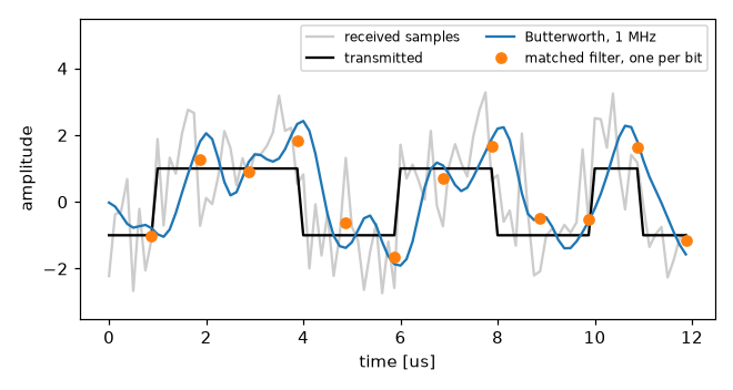
The formula assumes the best possible receiver. To check it, simulate the link at the baseband: each bit becomes 8 samples of +1 or -1, white Gaussian noise is added at a chosen \(E_b/N_0\), and the receiver decides each bit from the sign of a filtered sample. The optimum filter for a rectangular pulse is matched to it: average the 8 samples of each bit, which is a moving average read once per bit. 6 dB of \(E_b/N_0\), the link near 50 km, gives enough errors to count:

rng = np.random.default_rng(1)
n_bits, sps = 200_000, 8                       # bits, samples per bit
bits = rng.integers(0, 2, n_bits)
tx = np.repeat(cm.bpsk(bits).astype(float), sps)
ebn0 = cm.from_db(6.0)
N0 = sps / ebn0                                # Eb = sps for unit-amplitude samples
rx = tx + rng.normal(0, np.sqrt(N0 / 2), tx.size)

matched = sp.moving_average(rx, sps)[::sps]
ber_matched = np.mean((matched > 0) != bits)
print(f"matched filter: BER {ber_matched:.2e}, theory {cm.ber_bpsk_awgn(ebn0):.2e}")
# matched filter: BER 2.25e-03, theory 2.39e-03

Any other filter does worse. A fourth-order Butterworth low-pass, sampled at the best instant in each bit, loses to the matched filter however its cutoff is chosen: too narrow and each bit smears into the next (intersymbol interference), too wide and it lets in noise.

fs = sps * bit_rate
cutoffs = (0.5e6, 1e6, 2e6)
for fc in cutoffs:
    b, a = sp.butterworth_lowpass(4, fc, fs)
    y = sp.filter_signal(b, a, rx)
    best = min(np.mean((y[np.arange(n_bits) * sps + k] > 0) != bits) for k in range(sps))
    print(f"Butterworth, cutoff {fc / 1e6:.1f} MHz: BER {best:.2e}")
    assert best > ber_matched
# Butterworth, cutoff 0.5 MHz: BER 2.47e-01
# Butterworth, cutoff 1.0 MHz: BER 1.45e-02
# Butterworth, cutoff 2.0 MHz: BER 5.24e-02

fig, ax = plt.subplots(figsize=(6, 3.2))
t_us = np.arange(12 * sps) / fs * 1e6
ax.plot(t_us, rx[: 12 * sps], color="0.8", label="received samples")
ax.plot(t_us, tx[: 12 * sps], "k", label="transmitted")
b, a = sp.butterworth_lowpass(4, 1e6, fs)
ax.plot(t_us, sp.filter_signal(b, a, rx)[: 12 * sps], label="Butterworth, 1 MHz")
ax.step(t_us[sps - 1 :: sps], matched[:12], "o", where="post", label="matched filter, one per bit")
ax.set(xlabel="time [us]", ylabel="amplitude", ylim=(-3.5, 5.5))
ax.legend(fontsize=8, ncols=2)
fig.tight_layout()

../_images/radio_link_to_bit_errors-5.png

5. Does coding help?#

The Hamming(7,4) code sends 7 bits for every 4, and corrects any single error in each block of 7. The rate costs energy: at a fixed \(E_b/N_0\) per data bit, each coded bit gets only 4/7 of it, so the raw channel makes more errors before the decoder corrects them.

for ebn0_db_k in (4.0, 6.0, 8.0):
    e = cm.from_db(ebn0_db_k)
    data = rng.integers(0, 2, 400_000)
    code = cm.hamming74_encode(data)
    received = cm.bpsk(code) + rng.normal(0, np.sqrt(1 / (2 * e * 4 / 7)), code.size)
    decoded = cm.hamming74_decode((received > 0).astype(int)).data
    print(f"Eb/N0 {ebn0_db_k:.0f} dB: uncoded BER {cm.ber_bpsk_awgn(e):.2e}, Hamming(7,4) BER {np.mean(decoded != data):.2e}")
# Eb/N0 4 dB: uncoded BER 1.25e-02, Hamming(7,4) BER 1.59e-02
# Eb/N0 6 dB: uncoded BER 2.39e-03, Hamming(7,4) BER 2.24e-03
# Eb/N0 8 dB: uncoded BER 1.91e-04, Hamming(7,4) BER 1.38e-04

At 4 dB the code makes things worse, at 6 dB it barely breaks even, and only at 8 dB does it start to win. A short hard-decision code buys little; the gap to Shannon’s limit was only closed by long codes with soft decisions, decades later.

See also: the Telstar link budget, Kotel’nikov’s optimum receiver and Hamming code examples, and the Communications exercises exercises.