The Telstar satellite link budget

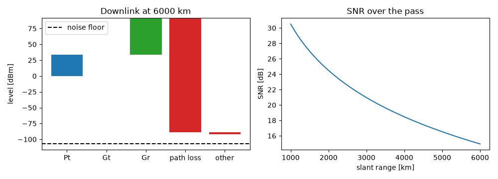
Telstar 1 (1962) relayed the first live transatlantic television. Engineers planned such links with a link budget: transmitter power, antenna gains, path loss and miscellaneous losses added in decibels (link_budget_db()), then compared with the receiver noise floor. The figures below are representative of the 4 GHz Andover-Telstar downlink, not archival values.

import matplotlib.pyplot as plt
import numpy as np

from engineeringkit.communications import (
    db,
    dbm,
    free_space_path_loss_db,
    friis_received_power,
    from_dbm,
    link_budget_db,
    thermal_noise_power,
)

Budget at the closest and farthest points of the orbit

pt_w, gt, gr, f = 2.25, 1.0, 10 ** (58 / 10), 4.17e9
bandwidth, t_sys = 25e6, 60.0
noise_dbm = float(dbm(thermal_noise_power(bandwidth, t_sys)))
ranges = np.linspace(1000e3, 6000e3, 60)
received = link_budget_db(float(dbm(pt_w)), float(db(gt)), float(db(gr)), free_space_path_loss_db(ranges, f), losses_db=3.0)
assert np.allclose(from_dbm(received + 3.0), friis_received_power(pt_w, gt, gr, ranges, f))
for r, p in [(ranges[0], received[0]), (ranges[-1], received[-1])]:
    print(f"range {r / 1e3:5.0f} km: received {p:6.1f} dBm, SNR {p - noise_dbm:5.1f} dB")

range  1000 km: received  -76.3 dBm, SNR  30.5 dB
range  6000 km: received  -91.9 dBm, SNR  14.9 dB

The decibel ledger

items = {
    "Pt": float(dbm(pt_w)),
    "Gt": float(db(gt)),
    "Gr": float(db(gr)),
    "path loss": -float(free_space_path_loss_db(ranges[-1], f)),
    "other": -3.0,
}
fig, axes = plt.subplots(1, 2, figsize=(10, 3.6))
running = np.cumsum(list(items.values()))
axes[0].bar(list(items), list(items.values()), bottom=np.r_[0, running[:-1]], color=["C0", "C2", "C2", "C3", "C3"])
axes[0].axhline(noise_dbm, color="k", ls="--", label="noise floor")
axes[0].set(ylabel="level [dBm]", title=f"Downlink at {ranges[-1] / 1e3:.0f} km")
axes[0].legend()
axes[1].plot(ranges / 1e3, received - noise_dbm)
axes[1].set(xlabel="slant range [km]", ylabel="SNR [dB]", title="SNR over the pass")
fig.tight_layout()

plt.show()