The Friis transmission formula

Harald Friis (1946) wrote the received power between two antennas in free space as \(P_r = P_t G_t G_r (\lambda/4\pi d)^2\) (friis_received_power()). The \(1/d^2\) factor is pure geometry: power spreads over a sphere of area \(4\pi d^2\). The \(\lambda^2\) factor comes from an antenna’s effective aperture, \(A_e = G\lambda^2/4\pi\). This example checks both interpretations and the 6 dB-per-doubling slope of free_space_path_loss_db().

import matplotlib.pyplot as plt
import numpy as np

from engineeringkit.communications import free_space_path_loss_db, friis_received_power, wavelength

Spherical spreading times effective aperture

Pt, Gt, Gr, f = 10.0, 30.0, 20.0, 5.8e9
d = np.logspace(2, 5, 100)
flux = Pt * Gt / (4 * np.pi * d**2)
aperture = Gr * float(wavelength(f)) ** 2 / (4 * np.pi)
assert np.allclose(friis_received_power(Pt, Gt, Gr, d, f), flux * aperture)

slope = np.polyfit(np.log2(d), free_space_path_loss_db(d, f), 1)[0]
print(f"path loss grows by {slope:.2f} dB per doubling of distance")
print(f"received power at 10 km: {float(friis_received_power(Pt, Gt, Gr, 1e4, f)) * 1e9:.2f} nW")

path loss grows by 6.02 dB per doubling of distance
received power at 10 km: 1.02 nW

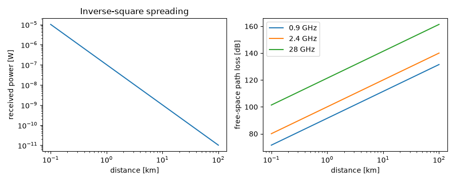
Higher frequency, same antennas: more loss

fig, axes = plt.subplots(1, 2, figsize=(9, 3.6))
axes[0].loglog(d / 1e3, friis_received_power(Pt, Gt, Gr, d, f))
axes[0].set(xlabel="distance [km]", ylabel="received power [W]", title="Inverse-square spreading")
for freq in [900e6, 2.4e9, 28e9]:
    axes[1].semilogx(d / 1e3, free_space_path_loss_db(d, freq), label=f"{freq / 1e9:g} GHz")
axes[1].set(xlabel="distance [km]", ylabel="free-space path loss [dB]")
axes[1].legend()
fig.tight_layout()

plt.show()