
Aerodynamics exercises#
Three problems built on the aerodynamics gallery. Try each one before opening its solution. The solutions run when the documentation is built, and the test suite checks every number they print.
1. Stall speed at altitude#
A light aircraft weighs 10.7 kN, has a wing area of 16.2 m² and a maximum lift coefficient of 1.6 with flaps. Find its stall speed at sea level and at 3000 m in the International Standard Atmosphere. By what factor does it rise, and why does the indicated airspeed at the stall not change?
Builds on: The Wright brothers, Smeaton’s coefficient and the stall speed and The International Standard Atmosphere.
Solution
import numpy as np

from engineeringkit.aerodynamics import isa_atmosphere, stall_speed

W, S, Clmax = 10.7e3, 16.2, 1.6
air = isa_atmosphere(np.array([0.0, 3000.0]))
vs = stall_speed(W, air.density, S, Clmax)
for h, rho, v in zip(air.altitude, air.density, vs):
    print(f"{h:4.0f} m: density {rho:.4f} kg/m^3, stall speed {v:.2f} m/s")
print(f"ratio {vs[1] / vs[0]:.4f}")
#    0 m: density 1.2250 kg/m^3, stall speed 25.96 m/s
# 3000 m: density 0.9091 kg/m^3, stall speed 30.14 m/s
# ratio 1.1608
assert np.isclose(vs[1] / vs[0], np.sqrt(air.density[0] / air.density[1]))
The true stall speed scales as \(1/\sqrt{\rho}\), 16% higher at 3000 m. The airspeed indicator measures dynamic pressure \(\tfrac12\rho V^2\), and the stall happens at the same dynamic pressure, \(W/(S\,C_{L,\max})\), at any altitude, so the indicated stall speed is the same.
2. The best glide#
A sailplane has a zero-lift drag coefficient of 0.012 and a wing of aspect ratio 20 with a span efficiency of 0.9. At what lift coefficient does it glide farthest, and what is its glide ratio? Check against the closed form \((L/D)_{\max} = \tfrac12\sqrt{\pi e AR/C_{D0}}\), and show that at the best glide the induced drag equals the zero-lift drag.
Builds on: Oswald’s efficiency factor and the parabolic drag polar.
Solution
import matplotlib.pyplot as plt
import numpy as np

from engineeringkit.aerodynamics import best_glide_cl, drag_polar, glide_ratio, induced_drag_coefficient

Cd0, AR, e = 0.012, 20.0, 0.9
cl_best = best_glide_cl(Cd0, AR, e)
ld_best = glide_ratio(cl_best, drag_polar(cl_best, Cd0, AR, e))
print(f"best-glide CL {cl_best:.3f}, glide ratio {ld_best:.1f}")
# best-glide CL 0.824, glide ratio 34.3
assert np.isclose(ld_best, 0.5 * np.sqrt(np.pi * e * AR / Cd0))
assert np.isclose(induced_drag_coefficient(cl_best, AR, e), Cd0)

cl = np.linspace(0.1, 1.6, 151)
fig, ax = plt.subplots(figsize=(5, 3.2))
ax.plot(cl, glide_ratio(cl, drag_polar(cl, Cd0, AR, e)))
ax.plot(cl_best, ld_best, "o")
ax.set(xlabel="lift coefficient", ylabel="L/D")
fig.tight_layout()
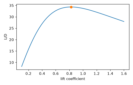
A glide ratio of 34 is typical of a club-class sailplane. Flying faster than the best glide (lower \(C_L\)) loses glide ratio slowly; flying slower loses it fast.
3. A normal shock in a supersonic intake#
Air at Mach 2 meets a normal shock. Find the Mach number and the static pressure ratio behind it. Then compare with the pressure recovered by an ideal isentropic diffuser: what fraction of the stagnation pressure does the shock destroy?
Builds on: Rankine-Hugoniot jump conditions across a normal shock and Saint-Venant and Wantzel: isentropic stagnation states.
Solution
import numpy as np

from engineeringkit.aerodynamics import normal_shock_mach2, normal_shock_pressure_ratio, stagnation_pressure

M1 = 2.0
M2 = normal_shock_mach2(M1)
p2_p1 = normal_shock_pressure_ratio(M1)
p01, p02 = stagnation_pressure(1.0, M1), stagnation_pressure(p2_p1, M2)
print(f"M2 = {M2:.4f}, p2/p1 = {p2_p1:.3f}")
print(f"stagnation pressure recovery p02/p01 = {p02 / p01:.4f}")
# M2 = 0.5774, p2/p1 = 4.500
# stagnation pressure recovery p02/p01 = 0.7209
assert np.isclose(M2, np.sqrt(1 / 3)) and np.isclose(p2_p1, 4.5)
The shock slows the flow to subsonic speed but destroys 28% of the stagnation pressure, which is why supersonic intakes slow the flow through a series of oblique shocks before a final weak normal one.