The International Standard Atmosphere

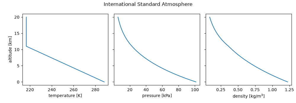
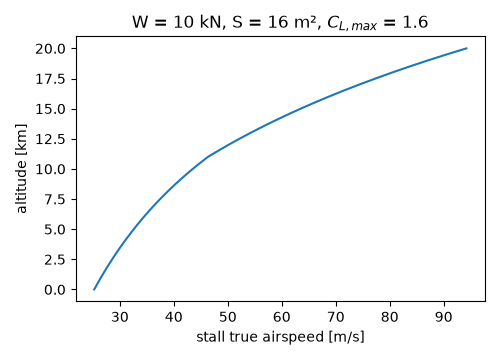
Aircraft performance depends on air density, which changes with weather. Albert Toussaint proposed a reference atmosphere in 1919, and ICAO adopted the International Standard Atmosphere in 1952: a 6.5 K/km linear lapse to the tropopause at 11 km, then an isothermal layer. Hydrostatic balance and the ideal-gas law give closed-form pressure and density (isa_atmosphere()). This example checks hydrostatic balance numerically and shows how thin air raises the stall speed.

import matplotlib.pyplot as plt
import numpy as np

from engineeringkit.aerodynamics import isa_atmosphere, stall_speed

Profiles and the hydrostatic check

h = np.linspace(0, 20000, 401)
state = isa_atmosphere(h)
residual = np.gradient(state.pressure, h) + state.density * 9.80665
print(f"max |dp/dh + rho g| / (rho g) = {np.max(np.abs(residual[1:-1] / (state.density[1:-1] * 9.80665))):.1e}")
for km in [0, 5, 11, 20]:
    s = isa_atmosphere(km * 1e3)
    print(f"{km:2d} km: T = {float(s.temperature):6.2f} K, p = {float(s.pressure):8.0f} Pa, rho = {float(s.density):.4f} kg/m^3")
fig, axes = state.plot()
fig.suptitle("International Standard Atmosphere")
fig.tight_layout()

max |dp/dh + rho g| / (rho g) = 3.7e-04
 0 km: T = 288.15 K, p =   101325 Pa, rho = 1.2250 kg/m^3
 5 km: T = 255.65 K, p =    54020 Pa, rho = 0.7361 kg/m^3
11 km: T = 216.65 K, p =    22632 Pa, rho = 0.3639 kg/m^3
20 km: T = 216.65 K, p =     5475 Pa, rho = 0.0880 kg/m^3

True stall speed rises with altitude

fig, ax = plt.subplots(figsize=(5, 3.6))
ax.plot(stall_speed(10_000.0, state.density, 16.0, 1.6), h / 1e3)
ax.set(xlabel="stall true airspeed [m/s]", ylabel="altitude [km]", title="W = 10 kN, S = 16 m², $C_{L,max}$ = 1.6")
fig.tight_layout()

plt.show()