Breakthroughs in Aerodynamics#
“It is possible to fly without motors, but not without knowledge and skill.” – attributed to Otto Lilienthal
Aerodynamics turned from speculation into engineering in about two
centuries. Bernoulli and Newton supplied the conservation laws; Cayley,
Lilienthal and the Wright brothers reduced flight to measurable force
coefficients; Kutta, Joukowski and Prandtl explained where lift and drag
come from; and the compressible-flow results of Saint-Venant, Rankine,
Hugoniot, Mach, de Laval, Fanno, Meyer and Rayleigh prepared the ground
for transonic and supersonic flight; and Glauert’s series and the panel
method of Hess and Smith turned the theory into computation. This chronology traces the ideas behind
engineeringkit.aerodynamics. Each entry links to the function that
implements the result and to a gallery example devoted to it.
1687-1816 – Newton, Laplace and the Speed of Sound#
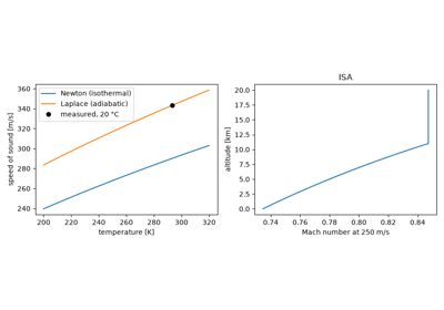
Book II of Isaac Newton’s Principia (1687) gave the first theory of sound: a pressure pulse travels at \(\sqrt{p/\rho}\). Newton assumed the compressions were isothermal, and his estimate came out about 15% below the measured value, a gap he papered over with unconvincing corrections. Pierre-Simon Laplace (1816) resolved it: the compressions are too fast for heat to flow, so they are adiabatic, and the gas’s stiffness is larger by the ratio of specific heats \(\gamma\). In a perfect gas the speed of sound becomes \(a = \sqrt{\gamma R T}\), and the Mach number \(M = V/a\) becomes the natural measure of compressibility.
Implementation: engineeringkit.aerodynamics.speed_of_sound() and
engineeringkit.aerodynamics.mach_number(). The example compares
Newton’s and Laplace’s predictions with the measured value at 20 °C.
References: I. Newton, Philosophiae Naturalis Principia Mathematica (London, 1687), Book II, Props. 48-50; P.-S. Laplace, “Sur la vitesse du son dans l’air et dans l’eau,” Annales de Chimie et de Physique 3 (1816) 238-241.
Newton, Laplace and the speed of sound (1687-1816)
1738 – Bernoulli’s Hydrodynamica and Dynamic Pressure#
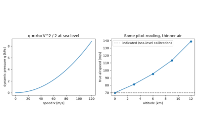
Daniel Bernoulli’s Hydrodynamica (1738) argued from the conservation of “live force” (kinetic energy) that the pressure in a moving fluid falls where its speed rises. Leonhard Euler later put the result in its modern form, \(p + \tfrac12\rho V^2 = \text{const}\) along a streamline of steady, inviscid, incompressible flow. The kinetic term \(q = \tfrac12\rho V^2\), the dynamic pressure, is the scale of every aerodynamic force, and the pitot-static tube that measures airspeed reads it directly.
Implementation: engineeringkit.aerodynamics.dynamic_pressure().
The example turns a fixed pitot reading into true airspeed at several
altitudes of the standard atmosphere.
References: D. Bernoulli, Hydrodynamica, sive de viribus et motibus fluidorum commentarii (Strasbourg, 1738); L. Euler, “Principes généraux du mouvement des fluides,” Mém. Acad. Sci. Berlin 11 (1757) 274-315.
Bernoulli’s dynamic pressure and the pitot-static airspeed (1738)
1809 – Cayley Separates Lift from Thrust#
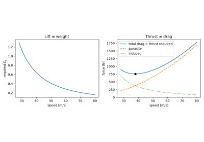
George Cayley’s three-part essay On Aerial Navigation (1809-1810) abandoned the flapping ornithopter for a fixed wing that supports the weight, plus a separate means of propulsion that overcomes the resistance. The idea seems obvious now but was revolutionary at the time: it splits the aerodynamic force into lift perpendicular to the flight path and drag along it, and reduces steady flight to two equilibria, lift equal to weight and thrust equal to drag. Cayley measured both forces on a whirling arm and flew man-carrying gliders built on the principle.
Implementation: engineeringkit.aerodynamics.lift() and
engineeringkit.aerodynamics.drag(). The example balances a light
aircraft at every speed and finds the minimum-drag speed, where parasite
drag equals lift-induced drag.
References: G. Cayley, “On Aerial Navigation,” Nicholson’s Journal of Natural Philosophy, Chemistry and the Arts 24 (1809) 164-174; 25 (1810) 81-87, 161-169.
Cayley’s separation of lift and drag in level flight (1809)
1839 – Saint-Venant and Wantzel: Isentropic Outflow#
Adhémar Barré de Saint-Venant and Pierre Wantzel measured air escaping from a pressurised reservoir through an orifice. They derived the first correct compressible form of Bernoulli’s equation by combining the energy equation with the adiabatic law \(p\rho^{-\gamma} = \text{const}\). In modern notation, the stagnation temperature and pressure of a perfect gas are \(T_0/T = 1 + \tfrac{\gamma-1}{2}M^2\) and \(p_0/p = (T_0/T)^{\gamma/(\gamma-1)}\). They also observed that the mass flow stops increasing once the downstream pressure falls below a critical value, the first sign of choked flow.
Implementation: engineeringkit.aerodynamics.stagnation_temperature()
and engineeringkit.aerodynamics.stagnation_pressure(), both built on
engineeringkit.aerodynamics.isentropic_factor(). The example shows
that the compressibility error of a Bernoulli pitot formula grows like
\(M^2/4\).
References: A. J. C. B. de Saint-Venant and L. Wantzel, “Mémoire et expériences sur l’écoulement de l’air,” Journal de l’École Polytechnique 16 (1839) 85-122.
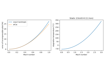
Saint-Venant and Wantzel: isentropic stagnation states (1839)
1870-1889 – Rankine and Hugoniot: the Shock Jump Conditions#
A shock wave is a discontinuity a few mean free paths thick, too thin for the inviscid equations to resolve. W. J. Macquorn Rankine (1870) and, independently, Pierre-Henri Hugoniot (1887-1889) sidestepped its structure by applying conservation of mass, momentum and energy across it. The resulting jump conditions fix the downstream state from the upstream Mach number alone. For a normal shock in a perfect gas they give \(p_2/p_1 = 1 + \tfrac{2\gamma}{\gamma+1}(M_1^2-1)\) and a subsonic downstream Mach number. Entropy rises across the shock, so only compression shocks are physical, and stagnation pressure is lost.
Implementation: engineeringkit.aerodynamics.normal_shock_mach2()
and engineeringkit.aerodynamics.normal_shock_pressure_ratio(). The
example rebuilds the downstream density, temperature and velocity and
checks all three conservation laws to round-off.
References: W. J. M. Rankine, “On the thermodynamic theory of waves of finite longitudinal disturbance,” Phil. Trans. R. Soc. 160 (1870) 277-288; H. Hugoniot, “Mémoire sur la propagation du mouvement dans les corps,” Journal de l’École Polytechnique 57 (1887) 3-97; 58 (1889) 1-125.
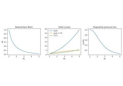
Rankine-Hugoniot jump conditions across a normal shock (1870-1889)
1883 – Reynolds and Dynamic Similarity#
Osborne Reynolds injected dye into water flowing through glass pipes and watched the streak stay straight at low speed and suddenly break up and fill the pipe at higher speed. The switch depended on the single combination \(\rho V D/\mu\), whatever the pipe or the fluid. Two geometrically similar flows with the same Reynolds number are dynamically similar. That principle makes wind-tunnel testing of scale models meaningful, and it led NACA to build its pressurised variable-density tunnel in 1923.
Implementation: engineeringkit.aerodynamics.reynolds_number(). The
example compares the Reynolds numbers of insects, birds and aircraft and
works out the tunnel pressure needed to test a 1/10-scale model at full
Reynolds number.
References: O. Reynolds, “An experimental investigation of the circumstances which determine whether the motion of water shall be direct or sinuous,” Phil. Trans. R. Soc. 174 (1883) 935-982.
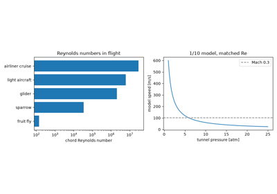
Reynolds’ dimensionless number and wind-tunnel similarity (1883)
1887 – Mach and Salcher Photograph a Supersonic Bullet#
Ernst Mach and Peter Salcher used spark-illuminated schlieren photography to capture a bullet in flight. Ahead of it was a curved bow shock, and trailing from it a conical wave whose half-angle satisfied \(\sin\mu = a/V\). A source moving faster than sound outruns its own wavefronts, so their envelope forms the Mach cone. Mach’s name was later given to the speed ratio \(M = V/a\) (by Jakob Ackeret, 1929).
Implementation: engineeringkit.aerodynamics.mach_angle(). The
example draws the wavefronts left behind by a subsonic, sonic and
supersonic source and checks that the envelope angle is
\(\arcsin(1/M)\).
References: E. Mach and P. Salcher, “Photographische Fixirung der durch Projectile in der Luft eingeleiteten Vorgänge,” Sitzungsberichte der Akademie der Wissenschaften Wien 95 (1887) 764-780.
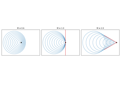
Ernst Mach’s shock photographs and the Mach cone (1887)
c. 1888 – De Laval’s Converging-Diverging Nozzle#
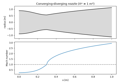
Gustaf de Laval needed very high steam velocities to drive his small impulse turbines. He found that a nozzle that first converges and then diverges delivers a supersonic jet, which a purely converging nozzle never can. Quasi-one-dimensional isentropic flow explains it. The area-velocity relation \(dA/A = (M^2-1)\,dV/V\) makes subsonic flow accelerate in a converging duct and supersonic flow accelerate in a diverging one, so the flow can pass through \(M = 1\) only at a throat. The area ratio \(A/A^*\) then fixes the Mach number at every station, on either a subsonic or a supersonic branch.
Implementation: engineeringkit.aerodynamics.area_mach_ratio(). The
example inverts the relation on both branches with a bracketing root
finder and traces the Mach number through a nozzle.
References: A. Stodola, Steam Turbines (New York: Van Nostrand, 1905), for de Laval’s nozzle; J. D. Anderson, Modern Compressible Flow, 3rd ed. (McGraw-Hill, 2003), ch. 5.
1889 – Lilienthal’s Coefficients and the Polar Diagram#
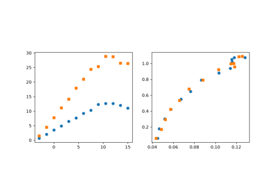
Otto Lilienthal measured the forces on cambered wings on a whirling arm and in the natural wind. He published the results in Der Vogelflug als Grundlage der Fliegekunst as tables of dimensionless coefficients and as a polar diagram of normal against tangential force. Dividing a force by \(qS\) removes its dependence on speed and size. Lilienthal then flew about two thousand glides on wings designed from these data before his fatal crash in 1896, and his tables were the starting point for the Wright brothers.
Implementation: engineeringkit.aerodynamics.lift_coefficient(),
engineeringkit.aerodynamics.drag_coefficient() and
engineeringkit.aerodynamics.glide_ratio(). The example reduces noisy
synthetic measurements at two arm speeds and shows them collapsing onto
one polar.
References: O. Lilienthal, Der Vogelflug als Grundlage der Fliegekunst (Berlin: Gaertner, 1889).
Lilienthal’s lift and drag coefficients and the polar diagram (1889)
1901 – The Wright Brothers Correct Smeaton’s Coefficient#
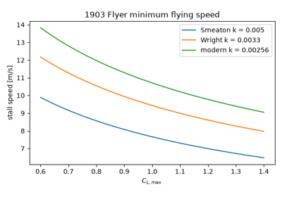
The Wrights’ 1901 glider produced only about a third of the lift predicted from Lilienthal’s tables and the lift equation \(L = kV^2SC_L\). That equation carried Smeaton’s 1759 air-pressure coefficient \(k = 0.005\) lb/(ft² mph²). In a home-built wind tunnel with balances that measured lift and drag ratios directly, the brothers tested about two hundred model wings and concluded that \(k\) was nearer 0.0033. The modern value, \(\tfrac12\rho\) at sea level, is 0.00256. With correct data they designed the 1903 Flyer’s wing and propellers by calculation.
Implementation: engineeringkit.aerodynamics.stall_speed(). The
example converts each historical \(k\) into an implied air density and
shows that Smeaton’s value under-predicts the Flyer’s minimum flying speed
by about 30%.
References: W. Wright, “Some Aeronautical Experiments,” Journal of the Western Society of Engineers 6 (1901) 489-510; M. W. McFarland (ed.), The Papers of Wilbur and Orville Wright (New York: McGraw-Hill, 1953).
The Wright brothers, Smeaton’s coefficient and the stall speed (1901)
1902-1906 – Kutta and Joukowski: Lift from Circulation#
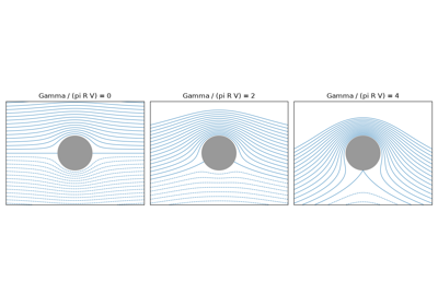
Martin Kutta (1902) and Nikolai Joukowski (1906) independently showed that the lift per unit span on a two-dimensional body in a steady inviscid stream is \(L' = \rho V \Gamma\). Here \(\Gamma\) is the circulation, the line integral of velocity around any closed curve enclosing the body. A sharp trailing edge fixes \(\Gamma\) through the Kutta condition: the flow must leave the edge smoothly. Potential flow could at last explain lift, though it still predicted zero drag (d’Alembert’s paradox).
Implementation: engineeringkit.aerodynamics.kutta_joukowski_lift().
The example integrates the Bernoulli surface pressure around a cylinder
with circulation and recovers \(\rho V\Gamma\) and zero drag to
round-off.
References: M. W. Kutta, “Auftriebskräfte in strömenden Flüssigkeiten,” Illustrierte Aeronautische Mitteilungen 6 (1902) 133-135; N. Joukowski, “Sur les tourbillons adjoints,” Bulletin de l’Institut Aérodynamique de Koutchino 1 (1906).
The Kutta-Joukowski theorem on a spinning cylinder (1902-1906)
1904 – Fanno: Friction Chokes a Duct#
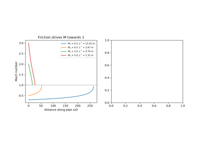
Gino Fanno’s diploma thesis at the ETH Zürich, written in 1904 under Aurel Stodola, followed an adiabatic gas along a constant-area pipe with wall friction. Friction does not slow a compressible flow down. It drives the Mach number towards one, accelerating subsonic flow and decelerating supersonic flow, while the stagnation temperature stays constant and the stagnation pressure falls. The states lie on a Fanno line whose point of maximum entropy is sonic, so a pipe longer than the choking length \(L^*\) cannot pass the inlet mass flow. Natural-gas pipelines and the ducts of supersonic wind tunnels are sized with it.
Implementation: engineeringkit.aerodynamics.fanno_flow() returns a
DuctFlowState, and
engineeringkit.aerodynamics.fanno_choking_length() gives \(L^*\).
The example marches the friction ODE down a pipe to the sonic point and
draws the Fanno line.
References: G. Fanno, Die Strömung eines Gases in einem Rohre mit Reibung, Diplomarbeit, ETH Zürich (1904); J. D. Anderson, Modern Compressible Flow, 3rd ed. (McGraw-Hill, 2003), sec. 3.9. The date and attribution follow Anderson; the thesis itself was not consulted.
1904-1908 – Prandtl’s Boundary Layer and the Blasius Solution#
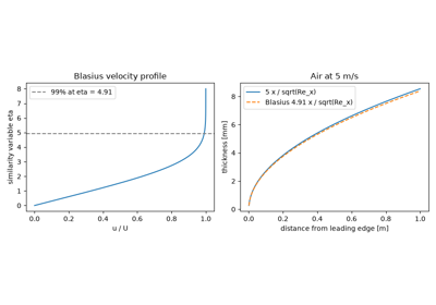
In an eight-page paper at the 1904 Heidelberg mathematics congress, Ludwig Prandtl argued that viscosity matters only in a thin boundary layer next to a surface, outside of which the flow is effectively inviscid. Within the layer the Navier-Stokes equations simplify. Prandtl’s student Heinrich Blasius (1908) found the similarity solution for a flat plate: the ODE \(f''' + \tfrac12 f f'' = 0\), whose wall shear gives \(C_f = 1.328/\sqrt{Re_L}\) and thickness \(\delta_{99} \approx 4.91\,x/\sqrt{Re_x}\). Boundary-layer theory resolved d’Alembert’s paradox and founded modern fluid mechanics.
Implementation: engineeringkit.aerodynamics.boundary_layer_laminar()
and engineeringkit.aerodynamics.skin_friction_laminar(). The example
solves the Blasius equation by shooting and recovers both constants.
References: L. Prandtl, “Über Flüssigkeitsbewegung bei sehr kleiner Reibung,” Verhandlungen des III. Internationalen Mathematiker-Kongresses, Heidelberg 1904 (Leipzig: Teubner, 1905) 484-491; H. Blasius, “Grenzschichten in Flüssigkeiten mit kleiner Reibung,” Zeitschrift für Mathematik und Physik 56 (1908) 1-37.
Prandtl’s boundary layer and the Blasius solution (1904-1908)
1907-1908 – The Prandtl-Meyer Expansion#
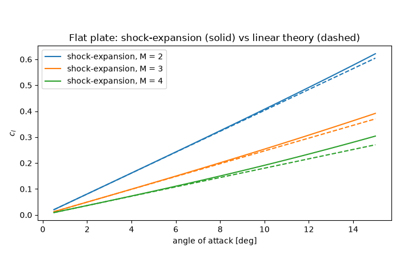
Ludwig Prandtl (1907), studying the supersonic jets from steam nozzles, and his student Theodor Meyer (1908) showed how a supersonic stream turns away from itself round a convex corner. It expands isentropically through a centred fan of Mach waves, and the turning angle that takes a sonic stream to Mach \(M\) is a single function \(\nu(M)\). A turn by \(\theta\) therefore sets \(\nu(M_2) = \nu(M_1) + \theta\). With Meyer’s oblique shocks this gives shock-expansion theory, the exact inviscid solution for supersonic airfoils made of straight segments.
Implementation: engineeringkit.aerodynamics.prandtl_meyer_angle(),
engineeringkit.aerodynamics.inverse_prandtl_meyer() and
engineeringkit.aerodynamics.prandtl_meyer_expansion(). The example
expands a Mach 1.5 stream round a 20° corner and computes the lift of a
flat plate by shock-expansion theory against Ackeret’s linear result.
References: L. Prandtl, “Neue Untersuchungen über die strömende Bewegung der Gase und Dämpfe,” Physikalische Zeitschrift 8 (1907) 23-30; T. Meyer, “Über zweidimensionale Bewegungsvorgänge in einem Gas, das mit Überschallgeschwindigkeit strömt,” Mitteilungen über Forschungsarbeiten auf dem Gebiete des Ingenieurwesens (VDI) 62 (1908) 31-67. The citations follow Anderson, Modern Compressible Flow, ch. 4; the original papers were not consulted.
1908 – Meyer’s Oblique Shock Relations#
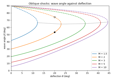
The same 1908 thesis treated the opposite case: a supersonic stream turned into itself by a wedge passes through a straight oblique shock. Meyer saw that the jump is a normal shock in the velocity component normal to the wave, while the tangential component is unchanged. That fixes the wave angle \(\beta\) from the deflection \(\theta\) and the Mach number through the \(\theta\)-\(\beta\)-\(M\) relation. For each Mach number there is a maximum deflection. Below it there are two solutions, a weak and a strong shock; above it the shock detaches and stands off the nose as a curved bow wave.
Implementation: engineeringkit.aerodynamics.oblique_shock_deflection(),
engineeringkit.aerodynamics.oblique_shock_angle() (Thompson’s closed
form for the cubic, 1950),
engineeringkit.aerodynamics.oblique_shock_max_deflection() and
engineeringkit.aerodynamics.oblique_shock(), which returns an
ObliqueShockResult. The chart is
drawn by engineeringkit.aerodynamics.visualizers.plot_theta_beta_mach().
The example finds both solutions for a 20° wedge at Mach 2.
References: T. Meyer, Mitteilungen über Forschungsarbeiten (VDI) 62 (1908) 31-67, as cited by J. D. Anderson, Modern Compressible Flow, 3rd ed. (McGraw-Hill, 2003), ch. 4; M. J. Thompson, “A note on the calculation of oblique shock-wave characteristics,” Journal of the Aeronautical Sciences 17 (1950) 744.
Meyer’s oblique shock and the theta-beta-M relation (1908)
1910 – Rayleigh Flow and Thermal Choking#
In “Aerial plane waves of finite amplitude,” Lord Rayleigh combined the conservation of mass and momentum for steady one-dimensional flow. The states they allow lie on a straight line, \(p + \rho V^2 =\) const, in the pressure-volume plane: the Rayleigh line. A gas heated or cooled in a frictionless constant-area duct moves along it. Heating drives the Mach number towards one from either side. The stagnation temperature is largest at the sonic point, so an inlet state can absorb only a finite heat before the duct chokes. That limit governs combustors, afterburners and ramjets.
Implementation: engineeringkit.aerodynamics.rayleigh_flow() and
engineeringkit.aerodynamics.rayleigh_choking_heat(). The example
checks mass and momentum along the line and finds its points of maximum
entropy (\(M = 1\)) and maximum temperature
(\(M = 1/\sqrt{\gamma}\)).
References: Lord Rayleigh, “Aerial plane waves of finite amplitude,” Proceedings of the Royal Society of London A 84 (1910) 247-284, doi:10.1098/rspa.1910.0075.
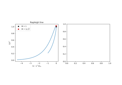
Rayleigh flow: heat addition and thermal choking (1910)
1918 – Prandtl’s Lifting-Line Theory#
A three-dimensional wing cannot carry lift up to its tips without shedding vorticity. Prandtl replaced the wing by a lifting line, a bound vortex of spanwise-varying strength, that sheds a sheet of trailing vortices. These induce a downwash that lowers each section’s effective angle of attack. The resulting integro-differential equation for the circulation distribution gives the finite-wing lift slope \(a = a_0/(1 + a_0/(\pi e AR))\). The slope approaches the 2-D value \(2\pi\) only as the aspect ratio becomes infinite.
Implementation: engineeringkit.aerodynamics.finite_wing_lift_slope()
and engineeringkit.aerodynamics.finite_wing_cl(). The example solves
Glauert’s Fourier form of the lifting-line equation for rectangular wings
and compares the computed slope with the closed form.
References: L. Prandtl, “Tragflügeltheorie,” Nachrichten von der Gesellschaft der Wissenschaften zu Göttingen, Math.-Phys. Klasse (1918) 451-477; (1919) 107-137.
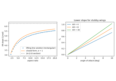
Prandtl’s lifting-line theory and the finite-wing lift slope (1918)
1918-1921 – Munk and the Minimum Induced Drag#
The downwash of the trailing vortices tilts each section’s lift backwards. The streamwise component is the induced drag, the price paid for generating lift with a finite span, and it equals \(C_L^2/(\pi e AR)\). Max Munk proved that for a given span and lift it is smallest when the downwash is uniform, which happens for an elliptic spanwise load (\(e = 1\)). Any other load shape adds harmonics and drag. The result explains the elliptic wings of the Supermarine Spitfire and the long, slender wings of sailplanes.
Implementation: engineeringkit.aerodynamics.induced_drag_coefficient().
The example computes \(e\) from the Fourier content of several
spanwise loads and confirms that the ellipse minimises induced drag.
References: M. M. Munk, “The minimum induced drag of aerofoils,” NACA Report 121 (1921).
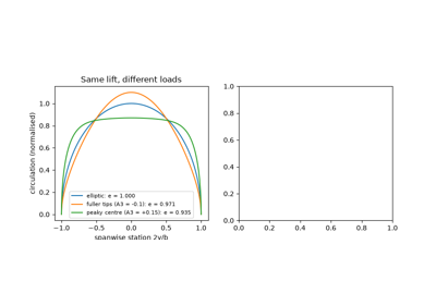
Induced drag and the optimality of elliptic loading (1918-1921)
1919-1952 – The Standard Atmosphere#
Aircraft performance depends on air density, which varies with weather and altitude, so test results could not be compared without a common reference. Albert Toussaint proposed one in France in 1919. NACA issued the first U.S. standard atmosphere in 1925, and the International Civil Aviation Organization adopted the International Standard Atmosphere in 1952. It assumes sea-level conditions of 288.15 K and 101325 Pa, a 6.5 K/km temperature lapse up to the tropopause at 11 km, and an isothermal layer above. Hydrostatic balance and the ideal-gas law then fix pressure and density in closed form.
Implementation: engineeringkit.aerodynamics.isa_atmosphere()
returns an AtmosphereState. The
example checks hydrostatic balance numerically and shows the stall speed
rising with altitude.
References: W. S. Diehl, “Standard atmosphere – tables and data,” NACA Report 218 (1925); ICAO, Manual of the ICAO Standard Atmosphere, Doc 7488 (1952); ISO 2533:1975.
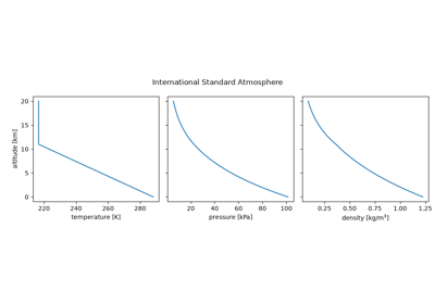
1922-1926 – Munk and Glauert: Thin-Airfoil Theory#
Munk (1922) modelled a thin section as a sheet of vortices along its camber line, and Hermann Glauert (1926) gave the theory its classical form with the change of variable \(x = \tfrac12(1-\cos\theta)\) and a Fourier series for the vortex strength. Two results stand out. Every thin section has the same lift slope, \(2\pi\) per radian. Camber only shifts the lift line, by a zero-lift angle given by an integral of the camber-line slope.
Implementation: engineeringkit.aerodynamics.thin_airfoil_cl() and
engineeringkit.aerodynamics.naca4_zero_lift_angle(), which evaluates
Glauert’s integral by quadrature, and
engineeringkit.aerodynamics.naca4_moment_coefficient() and
engineeringkit.aerodynamics.aerodynamic_center() for the pitching
moment, which is constant about the quarter chord. The first example
reproduces the textbook value \(\alpha_{L=0} = -2.08°\) for the NACA
2412; the second its \(c_{m,c/4} = -0.053\) and the aerodynamic
centre.
References: M. M. Munk, “General theory of thin wing sections,” NACA Report 142 (1922); H. Glauert, The Elements of Aerofoil and Airscrew Theory (Cambridge University Press, 1926).
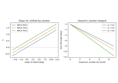
Thin-airfoil theory: lift slope 2π and the camber shift (1922-1926)
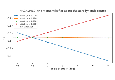
Thin-airfoil pitching moment and the aerodynamic centre (1922-1926)
c. 1920 – The Breguet Range Equation#
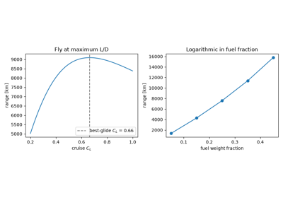
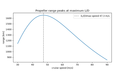
The range equation attributed to the French aviation pioneer Louis Breguet combines three facts about cruise. Thrust equals drag, drag equals weight divided by \(L/D\), and fuel burns at a rate set by the engine’s specific fuel consumption. Integrating the weight loss gives \(R = \frac{V}{g c_T}\frac{L}{D}\ln\frac{W_i}{W_f}\). Range is thus a product of three efficiencies: the engine’s, the airframe’s aerodynamics, and the structure’s (through the fuel fraction). The equation still frames every long-range aircraft design. Breguet wrote it for propeller aircraft, whose engines are rated by power rather than thrust. There \(R = \frac{\eta_{pr}}{g c_P}\frac{L}{D}\ln\frac{W_i}{W_f}\), and speed drops out.
Implementation: engineeringkit.aerodynamics.breguet_range(), with
engineeringkit.aerodynamics.best_glide_cl() giving the lift
coefficient that maximises \(L/D\), and
engineeringkit.aerodynamics.breguet_range_propeller(). The examples
check both forms against a time-stepped cruise.
References: J. D. Anderson, Aircraft Performance and Design (McGraw-Hill, 1999), sec. 5.13.
1926 – Glauert’s Fourier Solution of the Lifting Line#
Prandtl’s lifting-line equation could be solved by hand only for the elliptic wing. In The Elements of Aerofoil and Airscrew Theory Hermann Glauert turned it into linear algebra. He wrote the circulation as a Fourier sine series in the angle \(\theta\) with \(y = -\tfrac b2\cos\theta\), and enforced the equation at as many spanwise stations as there are terms. The first coefficient alone fixes the lift, \(C_L = \pi AR\,A_1\), and the others only add drag, so the span efficiency is \(e = 1/(1 + \delta)\) with \(\delta = \sum_{n>1} nA_n^2/A_1^2\). Glauert’s charts of \(\delta\) against taper ratio showed that a straight wing tapered to about 0.4 is almost as good as an ellipse and much easier to build.
Implementation: engineeringkit.aerodynamics.lifting_line() takes
any chord, twist and zero-lift distribution and returns a
LiftingLineResult, drawn by
engineeringkit.aerodynamics.visualizers.plot_spanwise_loading(). The
example recovers \(e = 1\) for the ellipse and sweeps the taper ratio.
References: H. Glauert, The Elements of Aerofoil and Airscrew Theory (Cambridge University Press, 1926), ch. 11; J. D. Anderson, Fundamentals of Aerodynamics, 6th ed. (McGraw-Hill, 2017), sec. 5.3.
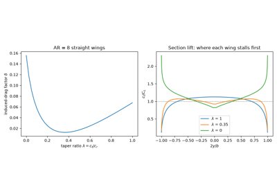
Glauert’s Fourier solution of the lifting line for any planform (1926)
1927 – Prandtl’s Turbulent Flat-Plate Friction#
Most aircraft surfaces carry turbulent boundary layers. Prandtl combined Blasius’s empirical pipe-friction law with a one-seventh-power velocity profile to estimate the friction on a turbulent flat plate, \(C_f = 0.074\,Re_L^{-1/5}\). It decays far more slowly with Reynolds number than the laminar law, so a turbulent layer can carry several times the friction drag. That is the reason behind later efforts to delay transition with laminar-flow airfoils.
Implementation: engineeringkit.aerodynamics.skin_friction_turbulent().
The example compares the laminar and turbulent laws and the mixed
friction of a plate that transitions part-way along.
References: L. Prandtl, “Über den Reibungswiderstand strömender Luft,” Ergebnisse der Aerodynamischen Versuchsanstalt zu Göttingen III (1927) 1-5; H. Schlichting and K. Gersten, Boundary-Layer Theory, 9th ed. (Springer, 2017), ch. 18.
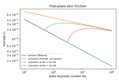
Turbulent skin friction and the one-fifth-power law (1927)
1928 – The Prandtl-Glauert Rule#
As propeller tips and then aircraft approached the speed of sound, pressure distributions measured at high subsonic speed no longer matched incompressible theory. Glauert showed that the linearised compressible potential equation reduces to Laplace’s equation in coordinates stretched by \(\sqrt{1-M_\infty^2}\). Every pressure coefficient and the lift slope are therefore amplified by \(1/\sqrt{1-M_\infty^2}\). The rule works well up to roughly Mach 0.7. Its divergence at \(M = 1\) fed the popular idea of a “sound barrier”.
Implementation: engineeringkit.aerodynamics.prandtl_glauert_cp().
The example compares it with the Kármán-Tsien rule (1939), which accounts
for part of the nonlinearity.
References: H. Glauert, “The effect of compressibility on the lift of an aerofoil,” Proc. R. Soc. Lond. A 118 (1928) 113-119; H. S. Tsien, “Two-dimensional subsonic flow of compressible fluids,” J. Aeronaut. Sci. 6 (1939) 399-407.
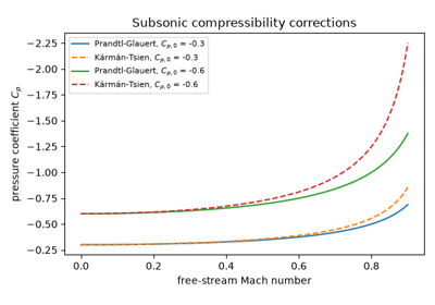
The Prandtl-Glauert compressibility correction (1928)
1933 – The NACA Four-Digit Sections#
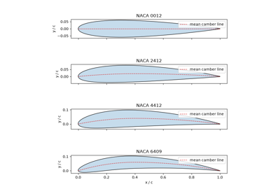
Before the 1930s, airfoils were drawn by hand and tested one at a time. Eastman Jacobs, Kenneth Ward and Robert Pinkerton defined a systematic family instead. A single thickness polynomial is laid perpendicular to a two-parabola camber line, so four digits specify the whole shape. They tested 78 related sections in the variable-density tunnel, making it possible to choose a section by its parameters. The NACA 0012 and 2412 are still used.
Implementation: engineeringkit.aerodynamics.naca4_airfoil()
returns an Airfoil, drawn by
engineeringkit.aerodynamics.visualizers.plot_airfoil(). The example
recovers each designation from the generated geometry.
References: E. N. Jacobs, K. E. Ward and R. M. Pinkerton, “The characteristics of 78 related airfoil sections from tests in the variable-density wind tunnel,” NACA Report 460 (1933).
1933 – Oswald’s Efficiency Factor and the Airplane Drag Polar#
W. Bailey Oswald’s NACA Report 408 extended the induced-drag formula from an isolated wing to a complete aeroplane. He absorbed the non-elliptic loading, the fuselage and the lift-dependent parasite drag into one empirical efficiency factor, \(e\), giving the parabolic polar \(C_D = C_{D0} + C_L^2/(\pi e AR)\). The polar puts aircraft performance in closed form. Maximum lift-to-drag occurs where induced drag equals parasite drag, at \(C_L = \sqrt{\pi e AR C_{D0}}\).
Implementation: engineeringkit.aerodynamics.drag_polar(),
engineeringkit.aerodynamics.oswald_efficiency_estimate() and
engineeringkit.aerodynamics.best_glide_cl(), plotted by
engineeringkit.aerodynamics.visualizers.plot_drag_polar(). The
example draws polars for three aspect ratios with their best-glide
tangents.
References: W. B. Oswald, “General formulas and charts for the calculation of airplane performance,” NACA Report 408 (1933).
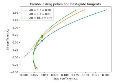
Oswald’s efficiency factor and the parabolic drag polar (1933)
1967 – Hess and Smith: the Panel Method#
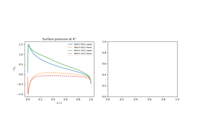
At the Douglas Aircraft Company, John Hess and A. M. O. Smith replaced a body of any shape by straight surface panels, each with its own uniform source strength, and solved the linear system that makes the surface a streamline. Their 1967 review added a vortex strength shared by every panel, fixed by the Kutta condition at the trailing edge, so the method could carry lift. It was among the first computational aerodynamics tools in industrial use. Unlike thin-airfoil theory it keeps the real thickness, and so predicts the leading-edge suction peak and the extra lift slope of a thick section. Panel methods were the industry’s workhorse until the 1980s and still size wings in conceptual design.
Implementation: engineeringkit.aerodynamics.panel_method()
returns a PanelResult, drawn by
engineeringkit.aerodynamics.visualizers.plot_pressure_coefficient().
The example matches the exact pressure on a circular cylinder and the
lift slope \(2\pi(1 + 0.77\,t/c)\) of symmetric NACA sections.
References: J. L. Hess and A. M. O. Smith, “Calculation of potential flow about arbitrary bodies,” Progress in Aerospace Sciences 8 (1967) 1-138, doi:10.1016/0376-0421(67)90003-6.