Bernoulli’s dynamic pressure and the pitot-static airspeed

Daniel Bernoulli’s Hydrodynamica (1738) traded pressure for speed along a streamline: \(p + \tfrac12\rho V^2\) is constant. A pitot tube brings the flow to rest and reads the total pressure; the static port reads \(p\); their difference is the dynamic pressure \(q = \tfrac12\rho V^2\) from dynamic_pressure(). Inverting it gives the airspeed, but only if the right density is used: the same pitot reading means a higher true airspeed at altitude.

import matplotlib.pyplot as plt
import numpy as np

from engineeringkit.aerodynamics import dynamic_pressure, isa_atmosphere

Dynamic pressure grows with the square of speed

V = np.linspace(0, 120, 121)
rho_sl = float(isa_atmosphere(0.0).density)
q = dynamic_pressure(rho_sl, V)
print(f"q at 50 m/s, sea level: {float(dynamic_pressure(rho_sl, 50.0)):.1f} Pa")

q at 50 m/s, sea level: 1531.3 Pa

The same pitot reading at altitude

Inverting Bernoulli, \(V = \sqrt{2q/\rho}\). An airspeed indicator is calibrated with sea-level density, so it shows the equivalent airspeed; the true airspeed is larger by \(\sqrt{\rho_0/\rho}\).

altitudes = np.array([0.0, 3000.0, 6000.0, 9000.0, 12000.0])
rho = isa_atmosphere(altitudes).density
q_reading = float(dynamic_pressure(rho_sl, 70.0))
true_speed = np.sqrt(2 * q_reading / rho)
for h, v in zip(altitudes, true_speed, strict=True):
    print(f"h = {h / 1e3:4.0f} km: indicated 70.0 m/s -> true {v:5.1f} m/s")
assert np.allclose(dynamic_pressure(rho, true_speed), q_reading)

fig, axes = plt.subplots(1, 2, figsize=(9, 3.5))
axes[0].plot(V, q / 1e3)
axes[0].set(xlabel="speed V [m/s]", ylabel="dynamic pressure q [kPa]", title="q = rho V^2 / 2 at sea level")
axes[1].plot(altitudes / 1e3, true_speed, "o-")
axes[1].axhline(70, color="gray", ls="--", label="indicated (sea-level calibration)")
axes[1].set(xlabel="altitude [km]", ylabel="true airspeed [m/s]", title="Same pitot reading, thinner air")
axes[1].legend()
fig.tight_layout()

plt.show()

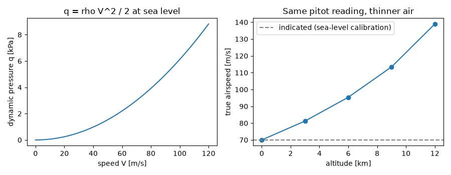
h =    0 km: indicated 70.0 m/s -> true  70.0 m/s
h =    3 km: indicated 70.0 m/s -> true  81.3 m/s
h =    6 km: indicated 70.0 m/s -> true  95.4 m/s
h =    9 km: indicated 70.0 m/s -> true 113.5 m/s
h =   12 km: indicated 70.0 m/s -> true 139.0 m/s