The Hess-Smith panel method (1967)

At the Douglas Aircraft Company, John Hess and A. M. O. Smith replaced a body by straight surface panels, each with its own uniform source strength, and solved for the strengths that make the surface a streamline. Their 1967 review in Progress in Aerospace Sciences added a single vortex strength shared by every panel. With the Kutta condition at the trailing edge, that let the method carry lift. panel_method() implements it. This example checks it against the exact flow round a circular cylinder, then shows what it adds to thin-airfoil theory: the leading-edge suction peak and the extra lift slope of a thick section.

import matplotlib.pyplot as plt
import numpy as np

from engineeringkit.aerodynamics import naca4_airfoil, panel_method, thin_airfoil_cl

The circular cylinder is exact

t = np.linspace(0, -2 * np.pi, 49)
circle = panel_method(np.column_stack((np.cos(t), np.sin(t))), 0.0)
angle = np.arctan2(circle.y, circle.x)
error = np.max(np.abs(circle.cp - (1 - 4 * np.sin(angle) ** 2)))
print(f"cylinder, 48 panels: max |Cp - (1 - 4 sin^2)| = {error:.1e}")
assert error < 1e-10

cylinder, 48 panels: max |Cp - (1 - 4 sin^2)| = 3.6e-15

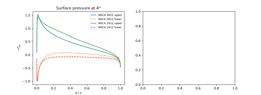
Pressure on the NACA 0012 and 2412

fig, axes = plt.subplots(1, 2, figsize=(11, 4))
for name in ("0012", "2412"):
    result = panel_method(naca4_airfoil(name, 101), np.radians(4.0))
    result.plot(ax=axes[0])
    axes[0].lines[-2].set_label(f"NACA {name} upper")
    axes[0].lines[-1].set_label(f"NACA {name} lower")
axes[0].set_title("Surface pressure at 4°")
axes[0].legend(fontsize=8)

<matplotlib.legend.Legend object at 0x7fa1ee1f7d40>

Lift slope grows with thickness

Thin-airfoil theory gives \(2\pi\) per radian whatever the thickness; the panel method gives about \(2\pi(1 + 0.77\,t/c)\).

alpha = np.radians(np.linspace(-4, 10, 8))
for name in ("0006", "0012", "0018"):
    cl = np.array([panel_method(naca4_airfoil(name, 101), a).cl for a in alpha])
    axes[1].plot(np.degrees(alpha), cl, "o-", ms=3, label=f"NACA {name}")
    slope = np.polyfit(alpha, cl, 1)[0]
    thickness = int(name[2:]) / 100
    print(f"NACA {name}: slope {slope:.3f} per rad = 2 pi x {slope / (2 * np.pi):.3f} (1 + 0.77 t/c = {1 + 0.77 * thickness:.3f})")
    assert np.isclose(slope, 2 * np.pi * (1 + 0.77 * thickness), rtol=0.02)
axes[1].plot(np.degrees(alpha), thin_airfoil_cl(alpha), "k--", label="thin airfoil, 2π")
axes[1].set(xlabel="angle of attack [deg]", ylabel="$c_l$", title="Inviscid lift of symmetric sections")
axes[1].legend()
fig.tight_layout()

plt.show()

NACA 0006: slope 6.571 per rad = 2 pi x 1.046 (1 + 0.77 t/c = 1.046)
NACA 0012: slope 6.828 per rad = 2 pi x 1.087 (1 + 0.77 t/c = 1.092)
NACA 0018: slope 7.094 per rad = 2 pi x 1.129 (1 + 0.77 t/c = 1.139)