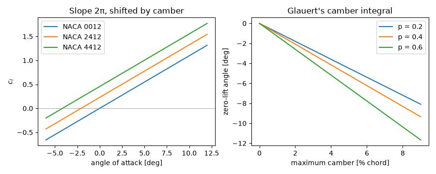
Thin-airfoil theory: lift slope 2π and the camber shift

Max Munk (1922) and Hermann Glauert (1926) replaced a thin section by a vortex sheet on its camber line. Satisfying flow tangency gives a lift slope of exactly \(2\pi\) per radian for every thin section, while camber only shifts the curve by a zero-lift angle given by an integral of the camber slope. naca4_zero_lift_angle() evaluates that integral for NACA four-digit camber lines, and thin_airfoil_cl() gives the lift line.

import matplotlib.pyplot as plt
import numpy as np

from engineeringkit.aerodynamics import naca4_zero_lift_angle, thin_airfoil_cl

Zero-lift angle versus camber

The integral is linear in the maximum camber m; moving the camber aft (larger p) makes it more negative.

for designation in ["0012", "2412", "4412", "4612"]:
    m, p = int(designation[0]) / 100, int(designation[1]) / 10 or 0.4
    a0 = float(naca4_zero_lift_angle(m, p))
    print(f"NACA {designation}: alpha_L=0 = {np.degrees(a0):+.2f} deg")
assert np.isclose(naca4_zero_lift_angle(0.04, 0.4), 2 * naca4_zero_lift_angle(0.02, 0.4))

NACA 0012: alpha_L=0 = -0.00 deg
NACA 2412: alpha_L=0 = -2.08 deg
NACA 4412: alpha_L=0 = -4.15 deg
NACA 4612: alpha_L=0 = -5.18 deg

Parallel lift lines

alpha = np.radians(np.linspace(-6, 12, 100))
fig, axes = plt.subplots(1, 2, figsize=(9, 3.6))
for designation in ["0012", "2412", "4412"]:
    m = int(designation[0]) / 100
    a0 = naca4_zero_lift_angle(m, 0.4)
    axes[0].plot(np.degrees(alpha), thin_airfoil_cl(alpha, a0), label=f"NACA {designation}")
axes[0].axhline(0, color="gray", lw=0.5)
axes[0].set(xlabel="angle of attack [deg]", ylabel="$c_l$", title="Slope 2π, shifted by camber")
axes[0].legend()

m_values = np.linspace(0, 0.09, 10)
for p in [0.2, 0.4, 0.6]:
    axes[1].plot(m_values * 100, [np.degrees(naca4_zero_lift_angle(m, p)) for m in m_values], label=f"p = {p}")
axes[1].set(xlabel="maximum camber [% chord]", ylabel="zero-lift angle [deg]", title="Glauert's camber integral")
axes[1].legend()
fig.tight_layout()

plt.show()