Lilienthal’s lift and drag coefficients and the polar diagram

Otto Lilienthal’s Der Vogelflug als Grundlage der Fliegekunst (1889) tabulated the forces on cambered wings measured on a whirling arm, reduced to dimensionless coefficients and plotted against each other in a polar diagram. Dividing a measured force by \(qS\) removes the dependence on speed and size, so tests at one speed predict forces at another. This example reduces synthetic whirling-arm measurements with lift_coefficient() and drag_coefficient() and reads the best glide ratio off the polar with glide_ratio().

import matplotlib.pyplot as plt
import numpy as np

from engineeringkit.aerodynamics import drag_coefficient, dynamic_pressure, glide_ratio, lift, lift_coefficient

Synthetic measurements at two arm speeds

A cambered plate with an assumed underlying behaviour is “measured” at 8 m/s and 12 m/s; the raw forces differ by a factor of 2.25.

rng = np.random.default_rng(1889)
alpha = np.radians(np.arange(-3, 16, 1.5))
true_cl = 0.3 + 4.6 * alpha - 6.0 * np.clip(alpha - np.radians(10), 0, None)
true_cd = 0.045 + 0.07 * true_cl**2
rho, S = 1.225, 0.3
fig, axes = plt.subplots(1, 2, figsize=(9, 3.8))
for V, marker in [(8.0, "o"), (12.0, "s")]:
    q = float(dynamic_pressure(rho, V))
    L = lift(q, S, true_cl) * (1 + 0.02 * rng.standard_normal(alpha.size))
    D = q * S * true_cd * (1 + 0.02 * rng.standard_normal(alpha.size))
    axes[0].plot(np.degrees(alpha), L, marker, label=f"lift at {V:.0f} m/s")
    cl = lift_coefficient(L, rho, V, S)
    cd = drag_coefficient(D, rho, V, S)
    axes[1].plot(cd, cl, marker, label=f"{V:.0f} m/s")
    best = int(np.argmax(glide_ratio(cl, cd)))
    print(f"{V:4.0f} m/s: best L/D = {glide_ratio(cl[best], cd[best]):.1f} at alpha = {np.degrees(alpha[best]):.1f} deg")

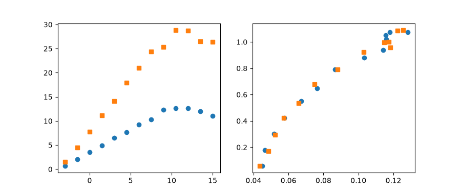
 8 m/s: best L/D = 9.1 at alpha = 6.0 deg
12 m/s: best L/D = 9.1 at alpha = 4.5 deg

Coefficients collapse both runs onto one polar

axes[0].set(xlabel="angle of attack [deg]", ylabel="measured lift [N]", title="Raw forces depend on speed")
axes[0].legend()
axes[1].set(xlabel="$C_D$", ylabel="$C_L$", title="Lilienthal's polar diagram")
axes[1].legend()
fig.tight_layout()

plt.show()