Induced drag and the optimality of elliptic loading

Prandtl and Max Munk (1918-1919) showed that the trailing vortices carry away kinetic energy at a rate that appears as an induced drag, \(C_{D,i} = C_L^2/(\pi e AR)\) (induced_drag_coefficient()), and that the elliptic spanwise load (\(e = 1\)) minimises it for a given span and lift. This example builds spanwise loads, computes their induced drag from the Fourier coefficients, and confirms the ellipse wins.

import matplotlib.pyplot as plt
import numpy as np

from engineeringkit.aerodynamics import induced_drag_coefficient

Span efficiency from the load shape

For \(\Gamma \propto \sum A_n \sin n\theta\) with lift fixed by \(A_1\), \(e = 1/(1 + \sum_{n>1} n A_n^2/A_1^2)\): any harmonic content beyond the ellipse adds drag.

theta = np.linspace(0, np.pi, 201)
y = -np.cos(theta)
loads = {"elliptic": [1.0, 0.0, 0.0], "fuller tips (A3 = -0.1)": [1.0, -0.1, 0.0], "peaky centre (A3 = +0.15)": [1.0, 0.15, 0.02]}
AR, CL = 8.0, 0.5
fig, axes = plt.subplots(1, 2, figsize=(9, 3.6))
for label, (a1, a3, a5) in loads.items():
    gamma = a1 * np.sin(theta) + a3 * np.sin(3 * theta) + a5 * np.sin(5 * theta)
    e = 1 / (1 + (3 * a3**2 + 5 * a5**2) / a1**2)
    axes[0].plot(y, gamma, label=f"{label}: e = {e:.3f}")
    print(f"{label:28s} e = {e:.4f}, C_Di = {float(induced_drag_coefficient(CL, AR, e)):.5f}")
axes[0].set(xlabel="spanwise station 2y/b", ylabel="circulation (normalised)", title="Same lift, different loads")
axes[0].legend(fontsize=8)

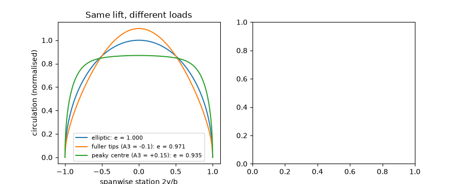
elliptic                     e = 1.0000, C_Di = 0.00995
fuller tips (A3 = -0.1)      e = 0.9709, C_Di = 0.01025
peaky centre (A3 = +0.15)    e = 0.9350, C_Di = 0.01064

<matplotlib.legend.Legend object at 0x7f0aec5e7110>

Induced drag grows with the square of lift

cl = np.linspace(0, 1.4, 50)
for ar in [5, 8, 12, 30]:
    axes[1].plot(cl, induced_drag_coefficient(cl, ar), label=f"AR = {ar}")
axes[1].set(xlabel="$C_L$", ylabel="$C_{D,i}$", title="Elliptic loading, e = 1")
axes[1].legend()
fig.tight_layout()

plt.show()