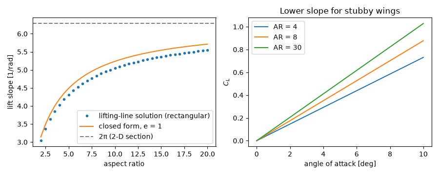
Prandtl’s lifting-line theory and the finite-wing lift slope

Ludwig Prandtl’s Tragflügeltheorie (1918) modelled a wing as a bound vortex of varying strength shedding a sheet of trailing vortices. The downwash they induce lowers the effective angle of attack, so a finite wing’s lift slope is \(a = a_0/(1 + a_0/(\pi e AR))\) (finite_wing_lift_slope()). This example solves Glauert’s Fourier form of the lifting-line equation for a rectangular wing and compares the computed slope with the closed form.

import matplotlib.pyplot as plt
import numpy as np

from engineeringkit.aerodynamics import finite_wing_cl, finite_wing_lift_slope

Solve the monoplane equation for a rectangular wing

With \(\Gamma = 2bV\sum A_n\sin n\theta\), collocation at stations \(\theta_k\) gives \(\sum_n A_n \sin n\theta_k\,(\mu n + \sin\theta_k) = \mu\alpha\sin\theta_k\) with \(\mu = a_0 c/(4b)\). Then \(C_L = \pi AR\,A_1\) and \(e = 1/(1 + \sum_{n>1} n A_n^2/A_1^2)\).

def rectangular_wing(AR, alpha=0.1, n_terms=15, a0=2 * np.pi):
    n = np.arange(1, 2 * n_terms, 2)
    theta = np.linspace(0, np.pi / 2, n_terms + 1)[1:]
    mu = a0 / (4 * AR)
    M = np.sin(np.outer(theta, n)) * (mu * n + np.sin(theta)[:, None])
    A = np.linalg.solve(M, mu * alpha * np.sin(theta))
    cl = np.pi * AR * A[0]
    e = 1 / (1 + np.sum(n[1:] * (A[1:] / A[0]) ** 2))
    return cl / alpha, e


aspect = np.linspace(2, 20, 37)
slopes, efficiencies = np.array([rectangular_wing(ar) for ar in aspect]).T
closed_form = finite_wing_lift_slope(aspect, efficiencies)
print(f"AR = 8 rectangular wing: e = {efficiencies[12]:.3f}, slope {slopes[12]:.3f} vs closed form {closed_form[12]:.3f} per rad")
# The closed form uses the drag-efficiency e in place of the lift-slope
# factor tau; they agree to within a few percent at moderate AR.
assert np.allclose(slopes, closed_form, rtol=0.03)

AR = 8 rectangular wing: e = 0.937, slope 4.838 vs closed form 4.959 per rad

Slope approaches 2π only as the span becomes infinite

fig, axes = plt.subplots(1, 2, figsize=(9, 3.6))
axes[0].plot(aspect, slopes, "o", ms=3, label="lifting-line solution (rectangular)")
axes[0].plot(aspect, finite_wing_lift_slope(aspect), label="closed form, e = 1")
axes[0].axhline(2 * np.pi, color="gray", ls="--", label="2π (2-D section)")
axes[0].set(xlabel="aspect ratio", ylabel="lift slope [1/rad]")
axes[0].legend()
alpha = np.radians(np.linspace(0, 10, 50))
for ar in [4, 8, 30]:
    axes[1].plot(np.degrees(alpha), finite_wing_cl(alpha, ar), label=f"AR = {ar}")
axes[1].set(xlabel="angle of attack [deg]", ylabel="$C_L$", title="Lower slope for stubby wings")
axes[1].legend()
fig.tight_layout()

plt.show()