Ernst Mach’s shock photographs and the Mach cone

In 1887 Ernst Mach and Peter Salcher photographed a supersonic bullet and saw a conical wave trailing from its nose. A source moving faster than sound outruns its own wavefronts; their envelope is a cone of half-angle \(\mu = \arcsin(1/M)\) (mach_angle()). This example draws the wavefronts emitted along the path and checks that the envelope matches the Mach angle.

import matplotlib.pyplot as plt
import numpy as np

from engineeringkit.aerodynamics import mach_angle

Wavefronts from a moving source

A pulse emitted at time \(t_i\) is a circle of radius \(a(t - t_i)\) centred where the source was.

a = 1.0
fig, axes = plt.subplots(1, 3, figsize=(11, 3.4))
for ax, M in zip(axes, [0.6, 1.0, 2.0], strict=True):
    t_now = 4.0
    for ti in np.arange(0, t_now, 0.4):
        circle = plt.Circle((M * a * ti, 0), a * (t_now - ti), fill=False, color="C0", lw=0.8)
        ax.add_patch(circle)
    x_src = M * a * t_now
    ax.plot(x_src, 0, "ko")
    if M >= 1:
        mu = mach_angle(M)
        length = 5
        ax.plot([x_src, x_src - length * np.cos(mu)], [0, length * np.sin(mu)], "C3")
        ax.plot([x_src, x_src - length * np.cos(mu)], [0, -length * np.sin(mu)], "C3")
        print(f"M = {M}: Mach angle {np.degrees(mu):.1f} deg")
    ax.set(xlim=(-4.5, 9), ylim=(-4.5, 4.5), title=f"M = {M}")
    ax.set_aspect("equal")
    ax.set_xticks([])
    ax.set_yticks([])
fig.tight_layout()

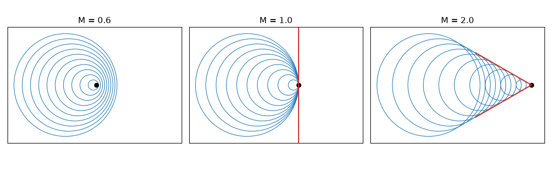
M = 1.0: Mach angle 90.0 deg
M = 2.0: Mach angle 30.0 deg

The envelope is the Mach cone

The tangent from the source to the oldest wavefront makes angle \(\arcsin(r/d) = \arcsin(a t/(M a t)) = \arcsin(1/M)\).

for M in [1.2, 2.0, 5.0]:
    d, r = M * a * 4.0, a * 4.0
    assert np.isclose(np.arcsin(r / d), mach_angle(M))

plt.show()