Meyer’s oblique shock and the theta-beta-M relation (1908)

Theodor Meyer’s 1908 Göttingen thesis showed that a supersonic stream turned into itself by a wedge passes through a straight oblique shock. Its wave angle \(\beta\) follows from the deflection \(\theta\) and the Mach number through the \(\theta\)-\(\beta\)-\(M\) relation (oblique_shock_deflection()). The jump itself is a normal shock in the velocity component normal to the wave (oblique_shock()). 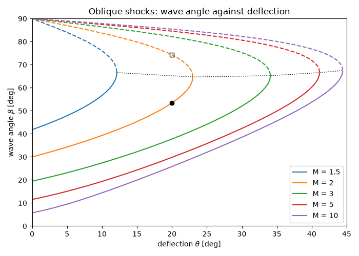This example draws the chart, finds the weak and strong solutions for a 20° wedge at Mach 2, and shows the shock detaching once the wedge is steeper than \(\theta_{\max}\).

import matplotlib.pyplot as plt
import numpy as np

from engineeringkit.aerodynamics import (
    normal_shock_mach2,
    oblique_shock,
    oblique_shock_deflection,
    oblique_shock_max_deflection,
)
from engineeringkit.aerodynamics.visualizers import plot_theta_beta_mach

Weak and strong solutions on a 20° wedge

theta = np.radians(20.0)
weak, strong = oblique_shock(2.0, theta), oblique_shock(2.0, theta, strong=True)
for name, shock in [("weak", weak), ("strong", strong)]:
    print(
        f"{name:6s}: beta = {np.degrees(shock.beta):5.2f} deg, M2 = {shock.mach2:.3f}, "
        f"p2/p1 = {shock.pressure_ratio:.3f}, p02/p01 = {shock.stagnation_pressure_ratio:.3f}"
    )
theta_max, beta_max = oblique_shock_max_deflection(2.0)
print(f"maximum deflection at M = 2: {np.degrees(theta_max):.2f} deg (beta = {np.degrees(beta_max):.2f} deg)")

# Both waves turn the flow by exactly 20°, and the normal component obeys the normal-shock law.
for shock in (weak, strong):
    assert np.isclose(oblique_shock_deflection(2.0, shock.beta), theta)
    assert np.isclose(shock.mach2 * np.sin(shock.beta - theta), normal_shock_mach2(2.0 * np.sin(shock.beta)))
assert weak.mach2 > 1 > strong.mach2

weak  : beta = 53.42 deg, M2 = 1.210, p2/p1 = 2.843, p02/p01 = 0.893
strong: beta = 74.27 deg, M2 = 0.728, p2/p1 = 4.157, p02/p01 = 0.756
maximum deflection at M = 2: 22.97 deg (beta = 64.67 deg)

The theta-beta-M chart

Solid curves are the weak branch seen on wedges and ramps; dashed curves the strong branch. To the right of the dotted line of maximum deflection no attached shock exists and a curved bow shock stands off the nose.

fig, ax = plt.subplots(figsize=(7, 5))
plot_theta_beta_mach([1.5, 2.0, 3.0, 5.0, 10.0], ax=ax)
ax.plot(np.degrees(theta), np.degrees(weak.beta), "ko")
ax.plot(np.degrees(theta), np.degrees(strong.beta), "ks", mfc="none")
ax.set(xlim=(0, 45), ylim=(0, 90), title="Oblique shocks: wave angle against deflection")
fig.tight_layout()

plt.show()