De Laval’s converging-diverging nozzle

Gustaf de Laval’s 1888 steam-turbine nozzle first converged and then diverged, and accelerated steam beyond the speed of sound. The quasi-one- dimensional isentropic relation \(A/A^*\) (area_mach_ratio()) explains why: subsonic flow speeds up in a converging duct, supersonic flow in a diverging one, and the sonic point sits at the throat. 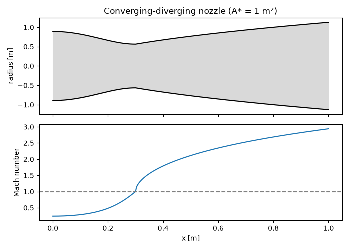Each area ratio has a subsonic and a supersonic solution; this example finds both with a root bracket and traces the Mach number through a nozzle.

import matplotlib.pyplot as plt
import numpy as np
from scipy.optimize import brentq

from engineeringkit.aerodynamics import area_mach_ratio

Invert A/A* on each branch

def mach_from_area(ratio, supersonic):
    lo, hi = (1.0, 50.0) if supersonic else (1e-6, 1.0)
    return brentq(lambda m: area_mach_ratio(m) - ratio, lo, hi)


for ratio in [1.0, 1.6875, 4.0]:
    sub, sup = mach_from_area(ratio, False), mach_from_area(ratio, True)
    print(f"A/A* = {ratio:6.4f}: subsonic M = {sub:.4f}, supersonic M = {sup:.4f}")
assert np.isclose(mach_from_area(1.6875, True), 2.0)

A/A* = 1.0000: subsonic M = 1.0000, supersonic M = 1.0000
A/A* = 1.6875: subsonic M = 0.3722, supersonic M = 2.0000
A/A* = 4.0000: subsonic M = 0.1465, supersonic M = 2.9402

Mach number along a nozzle

A cosine-shaped converging section to a throat at x = 0.3 m, then a conical diverging section to an exit area ratio of 4.

x = np.linspace(0, 1, 301)
throat = 0.3
area = np.where(x < throat, 1 + 1.5 * (1 + np.cos(np.pi * x / throat)) / 2, 1 + 3 * (x - throat) / (1 - throat))
mach = np.array([mach_from_area(ai, xi > throat) for xi, ai in zip(x, area, strict=True)])
fig, axes = plt.subplots(2, 1, figsize=(7, 5), sharex=True)
radius = np.sqrt(area / np.pi)
axes[0].fill_between(x, -radius, radius, color="0.85")
axes[0].plot(x, radius, "k", x, -radius, "k")
axes[0].set(ylabel="radius [m]", title="Converging-diverging nozzle (A* = 1 m²)")
axes[1].plot(x, mach)
axes[1].axhline(1, color="gray", ls="--")
axes[1].set(xlabel="x [m]", ylabel="Mach number")
fig.tight_layout()

plt.show()