The Kutta-Joukowski theorem on a spinning cylinder

Martin Kutta (1902) and Nikolai Joukowski (1906) showed that the lift per unit span on any two-dimensional body in a steady inviscid stream is \(L' = \rho V \Gamma\), where \(\Gamma\) is the circulation around the body (kutta_joukowski_lift()). The cleanest check is potential flow past a cylinder with circulation (a model of the Magnus effect): integrating the Bernoulli surface pressure around the cylinder reproduces \(\rho V\Gamma\) exactly, and the drag integrates to zero (d’Alembert’s paradox).

import matplotlib.pyplot as plt
import numpy as np
from scipy.integrate import quad

from engineeringkit.aerodynamics import dynamic_pressure, kutta_joukowski_lift

rho, V, R = 1.225, 20.0, 0.5

Integrate the surface pressure

On the surface the tangential speed is \(u_\theta = -2V\sin\theta - \Gamma/(2\pi R)\), and Bernoulli gives \(p - p_\infty = q\,(1 - u_\theta^2/V^2)\).

def surface_forces(gamma):
    q = float(dynamic_pressure(rho, V))

    def dp(theta):
        u = -2 * V * np.sin(theta) - gamma / (2 * np.pi * R)
        return q * (1 - (u / V) ** 2)

    lift_per_span = -quad(lambda t: dp(t) * np.sin(t) * R, 0, 2 * np.pi)[0]
    drag_per_span = -quad(lambda t: dp(t) * np.cos(t) * R, 0, 2 * np.pi)[0]
    return lift_per_span, drag_per_span


gammas = np.linspace(0, 4 * np.pi * R * V, 9)
integrated = np.array([surface_forces(g) for g in gammas])
theory = kutta_joukowski_lift(rho, V, gammas)
for g, (L, D), Lkj in zip(gammas, integrated, theory, strict=True):
    print(f"Gamma = {g:6.1f} m^2/s: integrated L' = {L:8.2f}, rho V Gamma = {Lkj:8.2f}, D' = {D:+.1e} N/m")
assert np.allclose(integrated[:, 0], theory, rtol=1e-9, atol=1e-9)
assert np.allclose(integrated[:, 1], 0, atol=1e-8)

Gamma =    0.0 m^2/s: integrated L' =     0.00, rho V Gamma =     0.00, D' = +1.0e-14 N/m
Gamma =   15.7 m^2/s: integrated L' =   384.85, rho V Gamma =   384.85, D' = +3.3e-14 N/m
Gamma =   31.4 m^2/s: integrated L' =   769.69, rho V Gamma =   769.69, D' = +3.2e-14 N/m
Gamma =   47.1 m^2/s: integrated L' =  1154.54, rho V Gamma =  1154.54, D' = +3.6e-14 N/m
Gamma =   62.8 m^2/s: integrated L' =  1539.38, rho V Gamma =  1539.38, D' = -1.3e-14 N/m
Gamma =   78.5 m^2/s: integrated L' =  1924.23, rho V Gamma =  1924.23, D' = +2.0e-14 N/m
Gamma =   94.2 m^2/s: integrated L' =  2309.07, rho V Gamma =  2309.07, D' = -5.4e-14 N/m
Gamma =  110.0 m^2/s: integrated L' =  2693.92, rho V Gamma =  2693.92, D' = -5.6e-14 N/m
Gamma =  125.7 m^2/s: integrated L' =  3078.76, rho V Gamma =  3078.76, D' = -6.0e-14 N/m

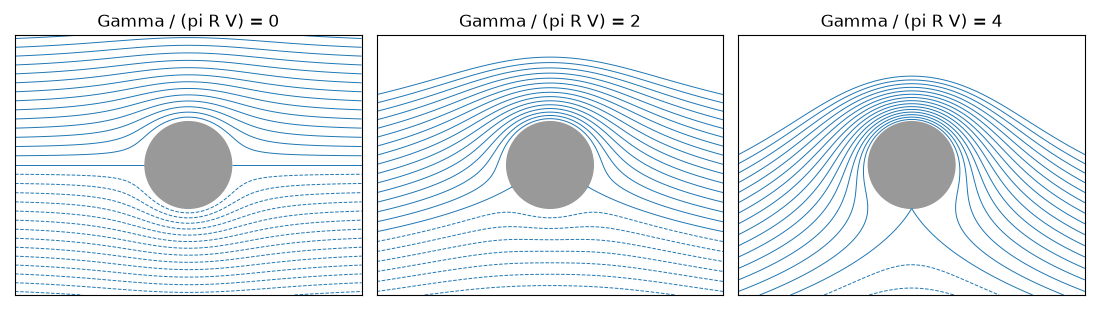
Streamlines with and without circulation

Circulation moves the stagnation points down; once \(\Gamma > 4\pi R V\) they leave the surface.

x, y = np.meshgrid(np.linspace(-2, 2, 400), np.linspace(-1.5, 1.5, 300))
r, th = np.hypot(x, y), np.arctan2(y, x)
fig, axes = plt.subplots(1, 3, figsize=(11, 3.3))
for ax, g in zip(axes, [0.0, 2 * np.pi * R * V, 4 * np.pi * R * V], strict=True):
    with np.errstate(divide="ignore"):
        psi = V * r * np.sin(th) * (1 - R**2 / r**2) + g / (2 * np.pi) * np.log(r / R)
    psi = np.where(r < R, np.nan, psi)
    ax.contour(x, y, psi, levels=np.linspace(-30, 30, 31), colors="C0", linewidths=0.7)
    ax.add_patch(plt.Circle((0, 0), R, color="0.6"))
    ax.set_aspect("equal")
    ax.set_title(f"Gamma / (pi R V) = {g / (np.pi * R * V):.0f}")
    ax.set_xticks([])
    ax.set_yticks([])
fig.tight_layout()

plt.show()