The Prandtl-Glauert compressibility correction

Hermann Glauert (1928), building on remarks by Prandtl, showed that the linearised subsonic potential equation is Laplace’s equation in stretched coordinates. Every pressure coefficient of a thin body is therefore amplified by \(1/\sqrt{1-M_\infty^2}\) (prandtl_glauert_cp()), a factor that blows up at \(M = 1\) and fed the myth of an impenetrable “sound barrier”. The Kármán-Tsien rule (1939) is plotted alongside: the two agree at low Mach and diverge as the flow becomes transonic.

import matplotlib.pyplot as plt
import numpy as np

from engineeringkit.aerodynamics import prandtl_glauert_cp

Amplification of a suction peak

M = np.linspace(0, 0.9, 181)
fig, ax = plt.subplots(figsize=(6, 4))
for cp0 in [-0.3, -0.6]:
    pg = prandtl_glauert_cp(cp0, M)
    beta = np.sqrt(1 - M**2)
    kt = cp0 / (beta + M**2 / (1 + beta) * cp0 / 2)
    ax.plot(M, pg, label=f"Prandtl-Glauert, $C_{{p,0}}$ = {cp0}")
    ax.plot(M, kt, "--", label=f"Kármán-Tsien, $C_{{p,0}}$ = {cp0}")
    print(f"C_p0 = {cp0}: at M = 0.7, PG {float(prandtl_glauert_cp(cp0, 0.7)):.3f}, KT {np.interp(0.7, M, kt):.3f}")
    assert np.isclose(pg[0], cp0)
ax.set(xlabel="free-stream Mach number", ylabel="pressure coefficient $C_p$", title="Subsonic compressibility corrections")
ax.invert_yaxis()
ax.legend(fontsize=8)
fig.tight_layout()

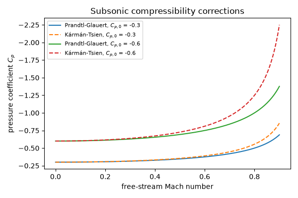
C_p0 = -0.3: at M = 0.7, PG -0.420, KT -0.447
C_p0 = -0.6: at M = 0.7, PG -0.840, KT -0.955

Lift slope rises the same way

The same factor multiplies the lift-curve slope: \(2\pi/\sqrt{1-M^2}\) is 25% higher at \(M = 0.6\).

print(f"lift-slope factor at M = 0.6: {float(prandtl_glauert_cp(1.0, 0.6)):.3f}")

plt.show()

lift-slope factor at M = 0.6: 1.250