Turbulent skin friction and the one-fifth-power law

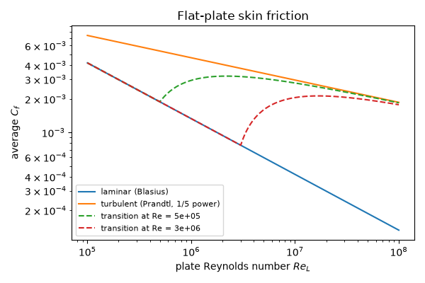
Prandtl (1927) carried Blasius’s empirical pipe-friction law over to the turbulent flat plate, with a \(u \propto y^{1/7}\) velocity profile. The result, \(C_f = 0.074\,Re_L^{-1/5}\) (skin_friction_turbulent()), decays far more slowly with Reynolds number than the laminar \(1.328\,Re_L^{-1/2}\); a turbulent layer can carry several times the friction drag. This example compares the two and the payoff of delaying transition.

import matplotlib.pyplot as plt
import numpy as np

from engineeringkit.aerodynamics import skin_friction_laminar, skin_friction_turbulent

Laminar versus turbulent friction coefficient

Re = np.logspace(5, 8, 200)
cf_lam = skin_friction_laminar(Re)
cf_turb = skin_friction_turbulent(Re)
for r in [5e5, 5e6, 5e7]:
    ratio = float(skin_friction_turbulent(r) / skin_friction_laminar(r))
    print(f"Re = {r:.0e}: turbulent / laminar C_f = {ratio:.1f}")
slope = np.polyfit(np.log(Re), np.log(cf_turb), 1)[0]
print(f"log-log slope of the turbulent law: {slope:.3f}")
assert np.isclose(slope, -0.2)

Re = 5e+05: turbulent / laminar C_f = 2.9
Re = 5e+06: turbulent / laminar C_f = 5.7
Re = 5e+07: turbulent / laminar C_f = 11.4
log-log slope of the turbulent law: -0.200

A laminar run before transition

A plate that stays laminar up to \(Re_{tr}\) then turns turbulent has \(C_f = 0.074/Re_L^{1/5} - A/Re_L\) with \(A = Re_{tr}(0.074\,Re_{tr}^{-1/5} - 1.328\,Re_{tr}^{-1/2})\).

fig, ax = plt.subplots(figsize=(6, 4))
ax.loglog(Re, cf_lam, label="laminar (Blasius)")
ax.loglog(Re, cf_turb, label="turbulent (Prandtl, 1/5 power)")
for re_tr in [5e5, 3e6]:
    A = re_tr * (skin_friction_turbulent(re_tr) - skin_friction_laminar(re_tr))
    mixed = np.where(Re < re_tr, cf_lam, cf_turb - A / Re)
    ax.loglog(Re, mixed, "--", label=f"transition at Re = {re_tr:.0e}")
ax.set(xlabel="plate Reynolds number $Re_L$", ylabel="average $C_f$", title="Flat-plate skin friction")
ax.legend(fontsize=8)
fig.tight_layout()

plt.show()