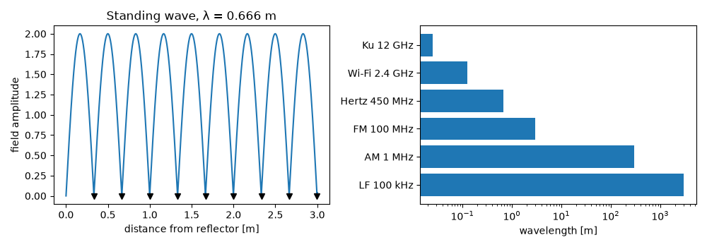
Hertz’s electromagnetic waves and their wavelength

Maxwell’s equations (1865) predicted electromagnetic waves travelling at the speed of light. Heinrich Hertz confirmed them in 1887-1888: a spark gap drove waves at a few hundred megahertz, a metal sheet reflected them into a standing wave, and the spacing of the nodes, half a wavelength, multiplied by the frequency gave the speed. wavelength() computes \(\lambda = c/f\); the example reconstructs Hertz’s standing-wave measurement and maps the radio spectrum.

import matplotlib.pyplot as plt
import numpy as np

from engineeringkit.communications import SPEED_OF_LIGHT, wavelength

A standing wave in front of a reflector

Incident and reflected waves add to \(2\sin(kx)\cos(\omega t)\); nodes are half a wavelength apart.

f = 450e6
lam = float(wavelength(f))
x = np.linspace(0, 3, 3001)
envelope = np.abs(2 * np.sin(2 * np.pi * x / lam))
interior = (envelope[1:-1] < envelope[:-2]) & (envelope[1:-1] < envelope[2:])
nodes = x[1:-1][interior]
spacing = np.mean(np.diff(nodes))
print(f"f = {f / 1e6:.0f} MHz: node spacing {spacing:.4f} m -> speed {2 * spacing * f:.4e} m/s (c = {SPEED_OF_LIGHT:.4e})")
assert np.isclose(2 * spacing * f, SPEED_OF_LIGHT, rtol=2e-3)

f = 450 MHz: node spacing 0.3331 m -> speed 2.9981e+08 m/s (c = 2.9979e+08)

Wavelengths across the radio spectrum

bands = {"LF 100 kHz": 1e5, "AM 1 MHz": 1e6, "FM 100 MHz": 1e8, "Hertz 450 MHz": 4.5e8, "Wi-Fi 2.4 GHz": 2.4e9, "Ku 12 GHz": 1.2e10}
fig, axes = plt.subplots(1, 2, figsize=(10, 3.5))
axes[0].plot(x, envelope)
axes[0].plot(nodes, np.zeros_like(nodes), "kv")
axes[0].set(xlabel="distance from reflector [m]", ylabel="field amplitude", title=f"Standing wave, λ = {lam:.3f} m")
axes[1].barh(list(bands), wavelength(np.array(list(bands.values()))))
axes[1].set_xscale("log")
axes[1].set(xlabel="wavelength [m]")
fig.tight_layout()

plt.show()