Jeffcott’s rotor and the critical speed (1919)

Rankine (1869) had argued that a shaft could not run stably above its whirling speed, yet de Laval’s steam turbines of the 1880s and 1890s did exactly that. Henry Jeffcott (1919) explained why with the simplest model: a disk whose centre of mass sits a small distance \(e\) from a flexible massless shaft. The shaft centre whirls in step with the spin at radius \(e r^2/\sqrt{(1 - r^2)^2 + (2\zeta r)^2}\), with \(r\) the speed over the critical speed \(\sqrt{k/m}\) (jeffcott_response()). 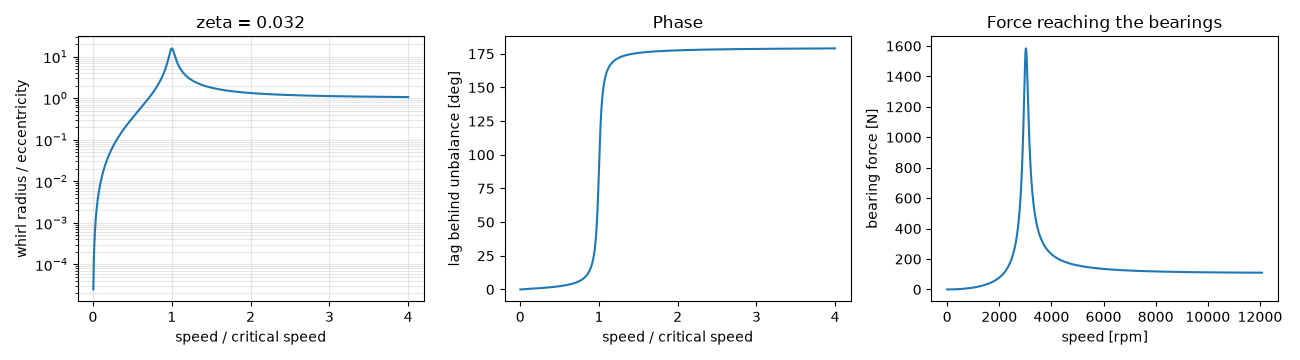Through resonance the whirl swings round by half a turn. Far above it the heavy side of the disk faces inward and the disk spins about its own centre of mass, so the whirl radius settles at \(e\). The force that reaches the bearings is the unbalance force (rotating_unbalance_force()) times the transmissibility (transmissibility()).

import matplotlib.pyplot as plt
import numpy as np

from engineeringkit.integrators import integrate_ode
from engineeringkit.mechanical_engineering import jeffcott_response, rotating_unbalance_force, transmissibility

m, k, e, c = 20.0, 2e6, 50e-6, 400.0
wc = np.sqrt(k / m)
zeta = c / (2 * np.sqrt(k * m))

Simulate the whirl

In complex coordinates \(z = x + iy\) the shaft centre obeys \(m\ddot z + c\dot z + kz = m e\omega^2 e^{i\omega t}\). Integrate from rest and compare the settled orbit with Jeffcott’s formula.

for ratio in (0.7, 1.0, 3.0):
    omega = ratio * wc
    t = np.linspace(0, 60 / zeta / wc, 40001)

    def rhs(tt, s, omega=omega):
        drive = m * e * omega**2 * np.array([np.cos(omega * tt), np.sin(omega * tt)])
        return [s[2], s[3], *((drive - c * s[2:] - k * s[:2]) / m)]

    orbit = integrate_ode(rhs, [0.0, 0.0, 0.0, 0.0], t).history
    radius = np.hypot(orbit[-2000:, 0], orbit[-2000:, 1]).mean()
    lag = np.angle(np.exp(1j * omega * t[-1]) / (orbit[-1, 0] + 1j * orbit[-1, 1]))
    theory = jeffcott_response(m, k, e, omega, c)
    print(
        f"r = {ratio}: simulated radius {1e6 * radius:7.2f} um, lag {np.degrees(lag):6.1f} deg; "
        f"Jeffcott {1e6 * float(theory.amplitude):7.2f} um, {np.degrees(float(theory.phase)):6.1f} deg"
    )
    assert np.isclose(radius, theory.amplitude, rtol=1e-3) and np.isclose(lag, theory.phase, atol=1e-3)

r = 0.7: simulated radius   47.86 um, lag    5.0 deg; Jeffcott   47.86 um,    5.0 deg
r = 1.0: simulated radius  790.57 um, lag   90.0 deg; Jeffcott  790.57 um,   90.0 deg
r = 3.0: simulated radius   56.23 um, lag  178.6 deg; Jeffcott   56.23 um,  178.6 deg

Self-centring and the bearing force

The bearing force \(|k + ic\omega|\,|z|\) equals \(m e\omega^2 T(r, \zeta)\).

speeds = np.linspace(0, 4 * wc, 801)
response = jeffcott_response(m, k, e, speeds, c)
bearing = np.abs(k + 1j * c * speeds) * response.amplitude
assert np.allclose(bearing, rotating_unbalance_force(m, e, speeds) * transmissibility(speeds / wc, zeta))
assert np.isclose(response.amplitude[-1] / e, 1, atol=0.08) and response.phase[-1] > np.radians(170)
print(response.summary())

fig, axes = plt.subplots(1, 3, figsize=(13, 3.6))
response.plot(ax=axes[0])
axes[0].set(title=f"zeta = {zeta:.3f}")
axes[1].plot(speeds / wc, np.degrees(response.phase))
axes[1].set(xlabel="speed / critical speed", ylabel="lag behind unbalance [deg]", title="Phase")
axes[2].plot(speeds * 60 / (2 * np.pi), bearing)
axes[2].set(xlabel="speed [rpm]", ylabel="bearing force [N]", title="Force reaching the bearings")
fig.tight_layout()

plt.show()

{'critical_speed_rad_s': 316.22776601683796, 'peak_amplitude_ratio': 15.811388300841898}