Armstrong’s wideband FM and Carson’s bandwidth rule

Edwin Howard Armstrong (1933-1936) demonstrated that frequency modulation with a deviation much larger than the message bandwidth trades bandwidth for a dramatic reduction of noise and static. The phase of an FM wave is the integral of the message (fm_signal()); for a tone of modulation index \(\beta = \Delta f/f_m\) the spectrum is a comb of Bessel-function sidebands \(J_n(\beta)\). Carson’s rule, \(B \approx 2(\Delta f + f_m)\) (carson_bandwidth()), captures about 98% of the power.

import matplotlib.pyplot as plt
import numpy as np
from scipy.special import jv

from engineeringkit.communications import carson_bandwidth, fm_signal

Bessel sidebands of a tone-modulated carrier

fs, fc, fm = 1.024e6, 100e3, 1e3
t = np.arange(0, 0.5, 1 / fs)
fig, axes = plt.subplots(1, 2, figsize=(10, 3.6))
for beta in [0.5, 5.0]:
    deviation = beta * fm
    s = fm_signal(np.cos(2 * np.pi * fm * t), t, fc, deviation)
    spectrum = np.abs(np.fft.rfft(s)) / (t.size / 2)
    freq = np.fft.rfftfreq(t.size, 1 / fs)
    n = np.arange(-12, 13)
    lines = spectrum[[np.argmin(np.abs(freq - (fc + k * fm))) for k in n]]
    assert np.allclose(lines, np.abs(jv(n, beta)), atol=2e-3)
    band = float(carson_bandwidth(deviation, fm))
    inside = np.abs(n) * fm <= band / 2
    share = np.sum(jv(n[inside], beta) ** 2)
    print(f"beta = {beta}: Carson bandwidth {band / 1e3:.0f} kHz holds {100 * share:.1f}% of the power")
    axes[0].stem(
        (fc + n * fm) / 1e3 + (0.1 if beta > 1 else -0.1), lines, markerfmt="o" if beta > 1 else "s", basefmt=" ", label=f"β = {beta}"
    )
axes[0].set(xlabel="frequency [kHz]", ylabel="line amplitude", title="Measured lines match |J_n(β)|")
axes[0].legend()

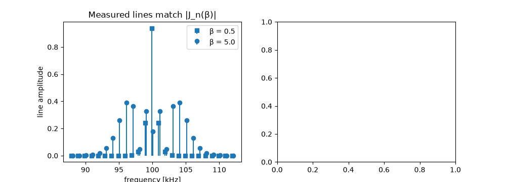
beta = 0.5: Carson bandwidth 3 kHz holds 99.8% of the power
beta = 5.0: Carson bandwidth 12 kHz holds 99.4% of the power

<matplotlib.legend.Legend object at 0x7f0af8783800>

Broadcast FM

75 kHz deviation with 15 kHz audio needs about 180 kHz; stations are spaced 200 kHz apart.

dev = np.linspace(0, 100e3, 101)
axes[1].plot(dev / 1e3, carson_bandwidth(dev, 15e3) / 1e3)
axes[1].plot(75, float(carson_bandwidth(75e3, 15e3)) / 1e3, "ko")
axes[1].set(xlabel="peak deviation [kHz]", ylabel="bandwidth [kHz]", title="Carson's rule, W = 15 kHz")
fig.tight_layout()

plt.show()