Kelvin’s telegraph cable and the RC time constant (1855)

Before the first transatlantic cable was laid, William Thomson (later Lord Kelvin) analysed how a signal spreads along a submarine cable. In 1855 he showed that, with negligible inductance, the line obeys a diffusion equation: a pulse arrives smeared over a time proportional to \(rc\,\ell^2\), the resistance and capacitance per unit length times the length squared, the law of squares. The building block is the single RC section, whose voltage rises as \(1 - e^{-t/RC}\) (rc_charging_voltage()). This example checks the time constant of one section, then chains sections into a cable and confirms the law of squares.

import matplotlib.pyplot as plt
import numpy as np

from engineeringkit.electrical_engineering import rc_charging_voltage, rc_time_constant

One RC section

R, C = 1e3, 1e-6
tau = rc_time_constant(R, C)
t = np.linspace(0, 5 * tau, 501)
v = rc_charging_voltage(1.0, R, C, t)
print(f"tau = {tau * 1e3:.1f} ms; v(tau) = {rc_charging_voltage(1.0, R, C, tau):.4f} (1 - 1/e = {1 - np.exp(-1):.4f})")
assert np.isclose(rc_charging_voltage(1.0, R, C, tau), 1 - np.exp(-1))

tau = 1.0 ms; v(tau) = 0.6321 (1 - 1/e = 0.6321)

A cable of N sections

A cable of length \(\ell\) is a ladder of RC sections; a unit step at the sending end reaches half amplitude at the far end (open circuit) after a delay that grows as \(\ell^2\) (here, the number of sections squared).

def far_end_half_time(n):
    """Far-end step response of n unit RC sections, by eigen-decomposition."""
    A = -2 * np.eye(n) + np.eye(n, k=1) + np.eye(n, k=-1)
    A[-1, -1] = -1.0  # the open far end has only one neighbour
    b = np.zeros(n)
    b[0] = 1.0
    lam, Q = np.linalg.eigh(A)  # A is symmetric
    x_final = -np.linalg.solve(A, b)
    times = np.linspace(0, 3 * n * n, 20001)
    far = x_final[-1] - (Q[-1] * (Q.T @ x_final)) @ np.exp(np.outer(lam, times))
    return times[np.argmax(far >= 0.5)], times, far


fig, axes = plt.subplots(1, 2, figsize=(10, 3.6))
axes[0].plot(t / tau, v)
axes[0].axhline(1 - np.exp(-1), color="gray", ls=":")
axes[0].set(xlabel="time / RC", ylabel="capacitor voltage [V]", title="One RC section")
sections = [10, 20, 40, 80]
delays = []
for n in sections:
    t_half, times, far = far_end_half_time(n)
    delays.append(t_half)
    axes[1].plot(times, far, label=f"{n} sections")
axes[1].set(xscale="log", xlabel="time / (r c)", ylabel="far-end voltage [V]", title="Signal smearing on a cable")
axes[1].legend()
fig.tight_layout()

exponent = np.polyfit(np.log(sections), np.log(delays), 1)[0]
print(f"delay grows as length^{exponent:.2f}")
assert abs(exponent - 2) < 0.05

plt.show()

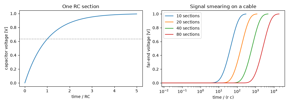
delay grows as length^1.96