Budeanu’s reactive power and the power factor (1927)

When a load’s current lags its voltage, part of the energy flows back and forth every half cycle and does no work. Constantin Budeanu of Bucharest gave this the name reactive power in 1927 and the unit “var” (volt-ampere reactive), adopted by the IEC in 1930. For sinusoids the power triangle holds: real power \(P = VI\cos\phi\) (real_power()), reactive power \(Q = VI\sin\phi\) (reactive_power()), apparent power \(S^2 = P^2 + Q^2\), and the power factor \(P/S\) (power_factor()). Budeanu extended \(Q\) to distorted waveforms as a sum over harmonics, which leaves a remainder he called the distortion power \(D\). This example checks the power triangle from waveforms and computes \(D\) for a current with harmonics.

import matplotlib.pyplot as plt
import numpy as np

from engineeringkit.electrical_engineering import power_factor, reactive_power, real_power, rms_sine

The power triangle from waveforms

V, I, phi, f = 230.0, 10.0, np.radians(40), 50.0
w = 2 * np.pi * f
t = np.linspace(0, 1 / f, 4000, endpoint=False)
v = np.sqrt(2) * V * np.cos(w * t)
i = np.sqrt(2) * I * np.cos(w * t - phi)
p = v * i
P, Q = real_power(V, I, np.cos(phi)), reactive_power(V, I, phi)
assert np.isclose(p.mean(), P)
# p(t) = P (1 + cos 2wt) + Q sin 2wt: Q is the amplitude of the energy that sloshes.
assert np.allclose(p, P * (1 + np.cos(2 * w * t)) + Q * np.sin(2 * w * t))
S = V * I
print(f"P = {P:.0f} W, Q = {Q:.0f} var, S = {S:.0f} VA, pf = {power_factor(P, S):.3f}")
assert np.isclose(S**2, P**2 + Q**2)

P = 1762 W, Q = 1478 var, S = 2300 VA, pf = 0.766

Distortion power

A rectifier-like load draws fifth and seventh harmonics from a sinusoidal supply. Only the fundamental carries real and reactive power, but the harmonics still raise the RMS current, so \(S^2 > P^2 + Q_B^2\).

harmonics = {1: (10.0, np.radians(20)), 5: (3.0, np.radians(-60)), 7: (2.0, np.radians(30))}
i_dist = sum(np.sqrt(2) * amp * np.cos(h * w * t - ph) for h, (amp, ph) in harmonics.items())
P_d = np.mean(v * i_dist)
Q_b = reactive_power(V, harmonics[1][0], harmonics[1][1])  # the voltage has no harmonics
S_d = V * np.sqrt(np.mean(i_dist**2))
D = np.sqrt(S_d**2 - P_d**2 - Q_b**2)
print(f"distorted load: P = {P_d:.0f} W, Q_B = {Q_b:.0f} var, D = {D:.0f} VA, pf = {power_factor(P_d, S_d):.3f}")
assert np.isclose(P_d, real_power(V, harmonics[1][0], np.cos(harmonics[1][1])))
assert np.isclose(D, V * np.hypot(3.0, 2.0))
assert np.isclose(rms_sine(np.sqrt(2) * V), V)

fig, axes = plt.subplots(1, 2, figsize=(10, 3.6))
axes[0].plot(t * 1e3, p / 1e3, label="p(t)")
axes[0].axhline(P / 1e3, color="C3", ls="--", label="P (average)")
axes[0].set(xlabel="time [ms]", ylabel="power [kW]", title="Real power and the sloshing part")
axes[0].legend()
axes[1].plot(t * 1e3, v / 100, label="v / 100")
axes[1].plot(t * 1e3, i_dist, label="distorted current")
axes[1].set(xlabel="time [ms]", ylabel="V / A", title="A harmonic-rich load")
axes[1].legend()
fig.tight_layout()

plt.show()

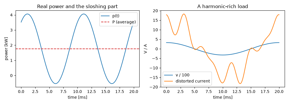
distorted load: P = 2161 W, Q_B = 787 var, D = 829 VA, pf = 0.884