Ward and Hale’s digital load flow (1956)

Until the 1950s, utilities computed the flow of power in their networks on AC network analysers, scale models of the grid built from resistors, inductors and capacitors. In 1956 J. B. Ward and H. W. Hale of American Gas and Electric published the first practical digital method. They wrote the network as its bus admittance matrix (admittance_matrix()) and improved each bus voltage in turn from the power specified there, a Gauss-Seidel iteration (gauss_seidel_load_flow()). 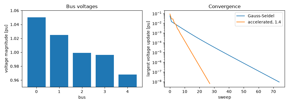The method is simple and needs little memory but converges slowly, which over-relaxation partly cures; Newton-Raphson methods replaced it in the 1960s. This example solves a five-bus network and checks the solution against a general-purpose nonlinear solver.

import matplotlib.pyplot as plt
import numpy as np
from scipy.optimize import root

from engineeringkit.electrical_engineering import admittance_matrix, gauss_seidel_load_flow

The network

Bus 0 is the slack (a large generator at 1.05 pu); buses 1-4 are loads, with bus 3 also hosting a generator that covers its 0.4 pu load. Line data are per unit on a 100 MVA base: series impedance and total line charging.

lines = [
    (0, 1, 0.02 + 0.06j, 0.06j),
    (0, 2, 0.08 + 0.24j, 0.05j),
    (1, 2, 0.06 + 0.18j, 0.04j),
    (1, 3, 0.06 + 0.18j, 0.04j),
    (2, 3, 0.01 + 0.03j, 0.02j),
    (3, 4, 0.04 + 0.12j, 0.03j),
]
Y = admittance_matrix(5, lines)
p_load = np.array([0.20, 0.45, 0.40 - 0.40, 0.40])
q_load = np.array([0.10, 0.15, 0.05, 0.10])

plain = gauss_seidel_load_flow(Y, p_load, q_load, v_slack=1.05)
fast = gauss_seidel_load_flow(Y, p_load, q_load, v_slack=1.05, acceleration=1.4)
for k, v in enumerate(plain.voltages):
    print(f"bus {k}: |V| = {abs(v):.4f} pu, angle {np.degrees(np.angle(v)):7.3f} deg")
print(f"slack generation {plain.power[0]:.4f} pu, losses {plain.losses.real * 100:.2f} MW")
print(f"sweeps: {plain.iterations} plain, {fast.iterations} with acceleration 1.4")
assert plain.converged and fast.converged and fast.iterations < plain.iterations / 2

bus 0: |V| = 1.0500 pu, angle   0.000 deg
bus 1: |V| = 1.0250 pu, angle  -2.082 deg
bus 2: |V| = 0.9990 pu, angle  -4.294 deg
bus 3: |V| = 0.9962 pu, angle  -4.517 deg
bus 4: |V| = 0.9680 pu, angle  -7.165 deg
slack generation 1.0863+0.2612j pu, losses 3.63 MW
sweeps: 75 plain, 28 with acceleration 1.4

An independent check

Solve the same power-balance equations, \(V_i (YV)_i^* = -S_i\), with SciPy’s hybrid Newton method from a flat start.

def mismatch(x):
    V = np.concatenate(([1.05], x[:4] + 1j * x[4:]))
    s = (V * (Y @ V).conj())[1:] + (p_load + 1j * q_load)
    return np.concatenate((s.real, s.imag))


check = root(mismatch, np.concatenate((np.ones(4), np.zeros(4))), tol=1e-12)
V_check = np.concatenate(([1.05], check.x[:4] + 1j * check.x[4:]))
assert check.success
assert np.allclose(plain.voltages, V_check, atol=1e-7)
assert np.isclose(plain.power[0].real, p_load.sum() + plain.losses.real)

fig, axes = plt.subplots(1, 2, figsize=(10, 3.6))
plain.plot(ax=axes[0])
axes[0].set(ylim=(0.95, 1.06), title="Bus voltages")
axes[1].semilogy(plain.history, label="Gauss-Seidel")
axes[1].semilogy(fast.history, label="accelerated, 1.4")
axes[1].set(xlabel="sweep", ylabel="largest voltage update [pu]", title="Convergence")
axes[1].legend()
fig.tight_layout()

plt.show()