
Breakthroughs in Semiclassical Physics#
“The most important application of the quantum theory… is that in which one lets Planck’s constant go to zero.” – paraphrasing the spirit of the WKB program
Semiclassical mechanics asks what quantum mechanics looks like in the
limit \(\hbar\to0\) without simply discarding quantum effects –
instead, it reorganizes them entirely around classical trajectories,
actions, and periodic orbits. This chronology traces that program behind
physicskit.semiclassical, from Weyl’s 1911 count of eigenvalues by
phase-space volume, through the WKB approximation, Feynman’s path
integral and Gutzwiller’s periodic orbits, to Bogomolny’s 1992 transfer
operator, with a pointer to the corresponding implementation in this
package at each stop.
1911 – Weyl’s Law#
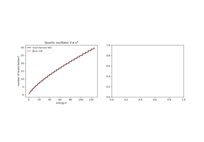
Hermann Weyl proved, in answer to a question Lorentz had raised in 1910, that the number of eigenvalues below \(k^2\) of the Laplacian on a two-dimensional membrane of area \(A\) grows as \(N(k)\simeq Ak^2/4\pi\), independent of the membrane’s shape (with \(Vk^3/6\pi^2\) for a three-dimensional cavity). Read semiclassically, the law says each quantum state occupies one cell of volume \((2\pi\hbar)^d\) in phase space, so the number of states below \(E\) is the phase-space volume enclosed by the energy surface divided by that cell size. This average level density is the smooth term that every later trace formula, from Balian-Bloch to Gutzwiller, adds its oscillations to.
Implementation: physicskit.semiclassical.core.wkb.wkb_action()
gives the phase-space area \(\oint p\,dx=2S(E)\) enclosed by a 1D
orbit, which counts the levels of a quartic oscillator;
physicskit.chaos.quantum.billiards.QuantumBilliard.weyl_counting_function()
applies the area law to billiards.
References: H. Weyl, “Über die asymptotische Verteilung der Eigenwerte,” Nachr. Ges. Wiss. Göttingen, Math.-Phys. Kl. 1911, 110-117 (1911); H. Weyl, “Das asymptotische Verteilungsgesetz der Eigenwerte linearer partieller Differentialgleichungen,” Math. Ann. 71, 441-479 (1912).
1917 – Einstein’s Torus Quantization#
The old quantum theory quantized each separated coordinate on its own, \(\oint p_i\,dq_i=n_ih\) (Sommerfeld, Wilson, Epstein), a rule whose result depended on which coordinates happened to separate. Albert Einstein replaced it with a coordinate-free condition: a multiply periodic motion winds around an invariant torus in phase space, and the quantization rule is one condition per independent closed loop on that torus, \(\oint_{\gamma_i}\mathbf p\cdot d\mathbf q=n_ih\). Because the loop integrals do not change when the loop is deformed on the torus, the rule needs no separable coordinates. Einstein also noted that a motion that fills a region of the energy surface, rather than a torus, admits no such rule, the first statement of the problem that chaotic systems pose for semiclassical quantization. Brillouin (1926) and Keller (1958) added the phase corrections that complete it into EBK quantization.
Example: the gallery example quantizes the two loops of the circular
billiard’s invariant tori, the angular action \(\hbar m\) and the
radial action between the caustic and the wall (with Keller’s offsets),
and compares the levels with the exact Bessel zeros. The 1D case of the
same rule is physicskit.semiclassical.core.wkb.bohr_sommerfeld_energies().
References: A. Einstein, “Zum Quantensatz von Sommerfeld und Epstein,” Verh. Dtsch. Phys. Ges. 19, 82-92 (1917); English translation in The Collected Papers of Albert Einstein, Vol. 6 (Princeton University Press, 1997), Doc. 45.
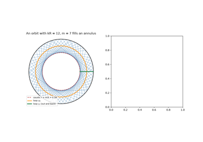
Einstein’s torus quantization: the circular billiard
1926 – The WKB Approximation#
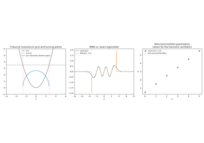
Gregor Wentzel, Hendrik Kramers, and Leon Brillouin (building on earlier work by Harold Jeffreys) independently found the leading term of an asymptotic expansion of the Schrodinger equation in powers of \(\hbar\): away from classical turning points, the wavefunction is well approximated by \(\psi(x)\sim p(x)^{-1/2}\exp(\pm i\int p\,dx/\hbar)\), an oscillation whose local wavelength and amplitude both track the classical momentum \(p(x)=\sqrt{2m(E-V(x))}\). Matching this oscillatory solution through the breakdown region at each turning point (via the Airy function) costs a phase of \(\pi/4\), and demanding the wavefunction close consistently around a full oscillation gives the Bohr-Sommerfeld quantization rule that had, until then, been an ad hoc postulate of the old quantum theory rather than a consequence of wave mechanics.
Implementation: physicskit.semiclassical.core.wkb.wkb_wavefunction()
builds exactly this approximate wavefunction;
bohr_sommerfeld_energies()
implements the resulting quantization condition, reproducing the exact
harmonic-oscillator spectrum to machine precision.
References: G. Wentzel, “Eine Verallgemeinerung der Quantenbedingungen für die Zwecke der Wellenmechanik,” Z. Phys. 38, 518-529 (1926); H. A. Kramers, “Wellenmechanik und halbzahlige Quantisierung,” Z. Phys. 39, 828-840 (1926); L. Brillouin, “La mécanique ondulatoire de Schrödinger: une méthode générale de resolution par approximations successives,” C. R. Acad. Sci. 183, 24-26 (1926); H. Jeffreys, “On Certain Approximate Solutions of Linear Differential Equations of the Second Order,” Proc. London Math. Soc. 23, 428-436 (1925).
1928 – Van Vleck’s Semiclassical Propagator#
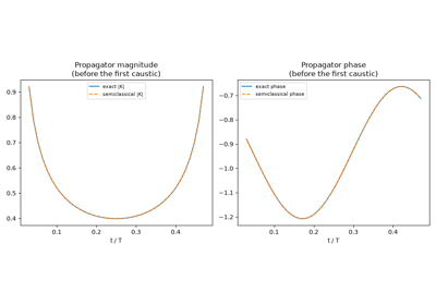
John Van Vleck showed that the WKB idea extends from stationary states to the full quantum propagator: the leading \(\hbar\to0\) approximation to \(K(x_f,t;x_i,0)\) is built entirely from a single classical trajectory connecting \(x_i\) to \(x_f\) in time \(t\), weighted by a prefactor set by that trajectory’s stability – how sensitively the endpoint depends on the launch momentum. Cecile Morette’s 1951 path-integral derivation later gave the same object a cleaner name, the Van Vleck-Morette determinant, and a systematic route to higher dimensions.
Implementation: physicskit.semiclassical.core.propagators.propagate_trajectory_monodromy_action()
integrates the classical trajectory together with its monodromy matrix;
van_vleck_propagator_1d()
assembles the propagator from it, matching the exact quantum propagator
of the free particle and the harmonic oscillator to better than
\(10^{-5}\).
plot_classical_trajectory_on_wigner()
overlays that same classical \((q,p)\) trajectory directly on the
exact quantum Wigner distribution, showing the classical orbit tracing
the ridge the quantum phase-space density concentrates on.
References: J. H. Van Vleck, “The Correspondence Principle in the Statistical Interpretation of Quantum Mechanics,” Proc. Natl. Acad. Sci. 14, 178-188 (1928); C. Morette, “On the Definition and Approximation of Feynman’s Path Integrals,” Phys. Rev. 81, 848-852 (1951).
1937 – The Langer Correction#
Applied to the radial equation of a central-force problem, the WKB rule gives the wrong energies, even for hydrogen. Rudolph Langer traced the error to the origin: near \(r=0\) the centrifugal term changes on the scale of the wavelength itself, so the WKB assumptions fail there. The substitution \(r=e^x\) maps the half-line onto the whole line, where WKB holds, and transforming back is equivalent to replacing \(l(l+1)\) by \((l+\tfrac12)^2\) in the centrifugal potential. With that change radial WKB gives the hydrogen spectrum \(-1/2(n_r+l+1)^2\) and the 3D oscillator spectrum exactly. The replacement reappears wherever angular momentum is quantized semiclassically, from atomic and nuclear physics to the angular phase of the torus quantization above.
Implementation: physicskit.semiclassical.core.wkb.langer_corrected_wkb()
solves the radial WKB condition with or without the correction, giving
the exact hydrogen levels with it and visibly wrong ones without.
References: R. E. Langer, “On the Connection Formulas and the Solutions of the Wave Equation,” Phys. Rev. 51, 669-676 (1937).
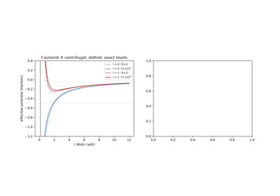
The Langer correction: exact hydrogen levels from radial WKB
1948 – Feynman’s Path Integral and the Classical Limit#
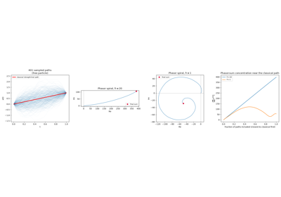
Building on Dirac’s 1933 remark that the quantum propagator over a short time behaves like \(\exp(iS/\hbar)\), Richard Feynman reformulated quantum mechanics as a sum over every path between two space-time points, each weighted by \(\exp(iS[x(t)]/\hbar)\) with \(S\) the classical action of that path. The formulation makes the classical limit transparent. Near the classical path the action is stationary, so neighbouring paths add in phase; far from it the phases vary rapidly and cancel. As \(\hbar\to0\) only the stationary path survives, and the principle of least action emerges from interference. Evaluating the path integral by stationary phase about that path gives back Van Vleck’s propagator, which is how Morette derived its determinant in 1951.
Implementation: physicskit.semiclassical.core.path_integral
samples random paths between fixed endpoints
(sample_random_paths()),
computes their discretized actions, and sums their phasors closest to
the classical path first
(build_phasor_diagram()),
for the free particle and the harmonic oscillator, whose classical paths
and actions are known in closed form.
References: P. A. M. Dirac, “The Lagrangian in Quantum Mechanics,” Phys. Z. Sowjetunion 3, 64-72 (1933); R. P. Feynman, “Space-Time Approach to Non-Relativistic Quantum Mechanics,” Rev. Mod. Phys. 20, 367-387 (1948); R. P. Feynman and A. R. Hibbs, Quantum Mechanics and Path Integrals (McGraw-Hill, New York, 1965).
1958 – Keller’s Quantization Condition and Maslov’s Topological Index#
Joseph Keller reformulated Bohr-Sommerfeld quantization for classically integrable systems with more than one degree of freedom, showing that the naive phase-space integral needs a correction term set by the number of caustics the trajectory crosses – turning points in 1D, or focal points more generally – each contributing a further \(-\pi/2\) to the phase. This “corrected Bohr-Sommerfeld” or Einstein-Brillouin-Keller (EBK) condition already contains, for the periodic-orbit case, the phase-counting rule that Viktor Maslov would later place on rigorous, coordinate-independent footing: in his 1965 monograph (English translation 1972), Maslov showed this phase count is a topological invariant of the trajectory – the Maslov index – rather than an artifact of the coordinates used to compute it, valid far beyond the periodic-orbit setting Keller started from.
Implementation: physicskit.semiclassical.core.propagators.count_caustics()
counts sign changes of the monodromy matrix’s \(\partial q_t/\partial p_0\)
element along a trajectory to extract exactly this index.
References: J. B. Keller, “Corrected Bohr-Sommerfeld Quantum Conditions for Nonseparable Systems,” Ann. Phys. 4, 180-188 (1958); V. P. Maslov, Théorie des Perturbations et Méthodes Asymptotiques (Dunod, Paris, 1972; Russian original, Moscow State University Press, 1965); V. P. Maslov and M. V. Fedoriuk, Semi-Classical Approximation in Quantum Mechanics (Reidel, Dordrecht, 1981).
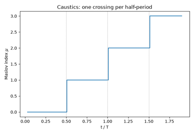
The Maslov index: caustics and Keller’s quantization condition
1971 – The Gutzwiller Trace Formula#
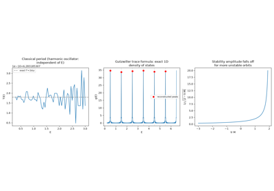
Martin Gutzwiller derived a semiclassical formula for the quantum density of states of a general – in particular, classically chaotic – system directly from its classical periodic orbits, with no reference to any quantum wavefunction at all: each isolated periodic orbit contributes an oscillatory term to \(g(E)\) at a frequency set by its action and an amplitude set by its linear instability. For chaotic systems, whose periodic orbits proliferate exponentially with period, the resulting sum is only conditionally convergent – famously “the most divergent series you’ll ever want to use” – yet reproduces real quantum spectra with striking accuracy when truncated sensibly.
Implementation: physicskit.semiclassical.core.gutzwiller.gutzwiller_density_of_states()
implements the exact bound-1D specialization of the trace formula (via
Poisson summation of the EBK spectrum), reconstructing the harmonic
oscillator’s Bohr-Sommerfeld levels from its classical action and period
alone; gutzwiller_amplitude_from_monodromy()
gives the general isolated-unstable-orbit stability amplitude the full
multi-dimensional formula uses.
References: M. C. Gutzwiller, “Periodic Orbits and Classical Quantization Conditions,” J. Math. Phys. 12, 343-358 (1971).
1972 – Balian and Bloch’s Level-Density Expansion#
In a series of papers from 1970 to 1972, Roger Balian and Claude Bloch expanded the Green function of the wave equation in a bounded domain as a series of multiple reflections off its boundary. The smooth part of the resulting level density is an asymptotic series in \(1/k\): Weyl’s area term, a perimeter correction \(\mp Lk/4\pi\) (minus for Dirichlet walls), then a constant set by corners and boundary curvature. The oscillating part, worked out in their third paper (1972), is a sum over the closed classical orbits of the billiard, each contributing a wave \(\cos(k\ell)\) at its length \(\ell\): a trace formula for billiards, derived independently of Gutzwiller’s from the wave equation rather than from the propagator.
Implementation: physicskit.semiclassical.core.gutzwiller.balian_bloch_counting_function()
evaluates the smooth series, including the corner and curvature
constant, and balian_bloch_level_density()
its derivative; for the disk and the rectangle the exact staircase
fluctuates about it with zero mean, and the Fourier transform of the
levels shows the periodic-orbit lengths.
References: R. Balian and C. Bloch, “Distribution of Eigenfrequencies for the Wave Equation in a Finite Domain. I. Three-Dimensional Problem with Smooth Boundary Surface,” Ann. Phys. 60, 401-447 (1970); R. Balian and C. Bloch, “Distribution of Eigenfrequencies for the Wave Equation in a Finite Domain. III. Eigenfrequency Density Oscillations,” Ann. Phys. 69, 76-160 (1972); H. P. Baltes and E. R. Hilf, Spectra of Finite Systems (Bibliographisches Institut, Mannheim, 1976).
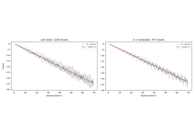
Balian and Bloch’s level-density expansion for billiards
1975 – Heller’s Thawed Gaussian Wavepackets#
Eric Heller proposed propagating a wavepacket by keeping it Gaussian and expanding the potential to second order about its moving centre. The Schrodinger equation then reduces to ordinary differential equations: the centre follows Hamilton’s equations, the complex width obeys a Riccati equation driven by the local curvature \(V''(q_t)\), and a phase collects the classical action. The width is free to breathe, squeeze and shear, in contrast to the fixed-width Gaussians of earlier classical trajectory methods. The method is exact for quadratic potentials and otherwise holds while the packet is small compared with the scale on which the curvature changes; as \(\hbar\to0\) with the classical motion fixed it converges to the exact result. It made semiclassical wavepacket dynamics a practical tool in chemical physics, and its failure for wide packets led to the multi-trajectory methods of Heller (1981) and Herman and Kluk (1984).
Implementation: physicskit.semiclassical.core.propagators.thawed_gaussian_propagate()
integrates the centre, the width (in the equivalent linear tangent-map
form, which stays regular where the Riccati equation is stiff) and the
phase; thawed_gaussian_wavefunction()
evaluates the packet on a grid.
References: E. J. Heller, “Time-Dependent Approach to Semiclassical Dynamics,” J. Chem. Phys. 62, 1544-1555 (1975).
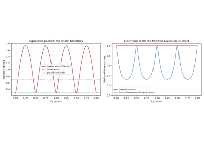
1976 – The Berry-Tabor Formula for Integrable Systems#
Michael Berry and Michael Tabor showed that the Gutzwiller trace formula’s assumption of isolated periodic orbits fails for integrable systems – where, since every energy has a whole torus of orbits rather than one isolated orbit, the trace formula must be replaced by a different (still exact, for linear tori) sum organized around rational winding numbers. The distinction between the Gutzwiller (chaotic, isolated orbits) and Berry-Tabor (integrable, orbit families) regimes remains the basic dichotomy of semiclassical spectral theory.
Connection: the one-dimensional trace formula in this package is the
\(f=1\) special case where the distinction is moot (a single degree
of freedom has no room for chaos), which is exactly why
gutzwiller_density_of_states()
can be exact rather than merely leading-order in \(\hbar\).
References: M. V. Berry and M. Tabor, “Closed Orbits and the Regular Bound Spectrum,” Proc. R. Soc. Lond. A 349, 101-123 (1976).
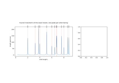
The Berry-Tabor formula: an integrable billiard’s spectrum
1977 – Berry’s Random-Wave Conjecture#
Michael Berry asked what a high-lying eigenfunction of a classically chaotic system looks like. The Wigner function of an eigenstate concentrates, semiclassically, on the part of phase space the classical motion at that energy explores. For an integrable system this is a torus, and the eigenfunction is ordered, with caustics and regular nodal patterns. For an ergodic system it is the whole energy surface, so at each point every momentum direction is equally likely, and Berry conjectured that the eigenfunction looks locally like a random superposition of plane waves of fixed wavenumber. Two predictions follow: Gaussian-distributed amplitudes, and a spatial autocorrelation \(J_0(k|\Delta\mathbf r|)\) in two dimensions. The conjecture is the eigenfunction counterpart of the random-matrix description of chaotic spectra; quantum scars (1984, below) are its best-known exceptions.
Example: the gallery example tests both predictions on Bunimovich
stadium eigenstates from
physicskit.chaos.quantum.billiards.QuantumBilliard, and
contrasts them with a disk eigenstate.
References: M. V. Berry, “Regular and Irregular Semiclassical Wavefunctions,” J. Phys. A 10, 2083-2091 (1977).
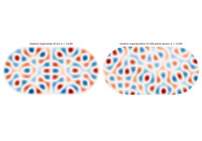
Berry’s random-wave conjecture for chaotic eigenfunctions
1978 – The Ehrenfest Time#
Ehrenfest’s theorem keeps a narrow wavepacket on a classical trajectory only while it stays narrow. Gennady Berman and George Zaslavsky asked how long that lasts when the classical motion is chaotic. A minimum-uncertainty packet starts with width of order \(\sqrt\hbar\); chaotic stretching grows it as \(e^{\lambda t}\), with \(\lambda\) the Lyapunov exponent, until it reaches the size of the system after a time of order \(\lambda^{-1}\ln(1/\hbar)\). This logarithmic time is very short: for a chaotic system, quantum-classical correspondence for individual trajectories fails long before the power-law times that apply to integrable motion. Berry, Balazs, Tabor and Voros found the same time scale in quantized maps in 1979. Beyond it, quantum averages can still follow classical ensemble averages, which is why the Ehrenfest time reappears in decoherence, weak localization and the growth of out-of-time-order correlators.
Example: the gallery example measures the time at which a coherent
state of physicskit.chaos.quantum.maps.QuantumKickedRotor
leaves the classical orbit of
physicskit.chaos.systems.maps.StandardMap, and finds it growing
as \(\ln(1/\hbar)/2\lambda\).
References: G. P. Berman and G. M. Zaslavsky, “Condition of Stochasticity in Quantum Nonlinear Systems,” Physica A 91, 450-460 (1978); M. V. Berry, N. L. Balazs, M. Tabor, and A. Voros, “Quantum Maps,” Ann. Phys. 122, 26-63 (1979).
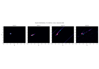
The Ehrenfest time: the log(1/ħ) breakdown of correspondence
1981 – Heller’s Time-Dependent Semiclassical Spectroscopy#
Eric Heller recast spectroscopy in the time domain. An absorption spectrum is the Fourier transform of the autocorrelation \(\langle\psi_0|\psi(t)\rangle\) of the wavepacket the transition creates, so each feature of the spectrum corresponds to an event in the packet’s motion at the reciprocal time scale: the initial decay as the packet leaves the Franck-Condon region sets the width of the band, the first return after a vibrational period splits it into a progression, and only long-time recurrences resolve single lines. Since the first two events take a period or two, short-time semiclassical dynamics, often a single thawed Gaussian, already explains the band shape and the progression. The same reasoning, applied to a packet launched along an unstable periodic orbit, is what led Heller to scars three years later.
Implementation: the example drops a ground-state packet onto a bound
(Morse) and a repulsive upper surface, propagates it with a single
physicskit.semiclassical.core.propagators.thawed_gaussian_propagate(),
and compares the Fourier-transformed autocorrelation with exact
Franck-Condon factors and with split-operator evolution
(physicskit.quantum.core.solvers.SplitOperatorSolver1D).
References: E. J. Heller, “The Semiclassical Way to Molecular Spectroscopy,” Acc. Chem. Res. 14, 368-375 (1981); E. J. Heller, “Quantum Corrections to Classical Photodissociation Models,” J. Chem. Phys. 68, 2066-2075 (1978).
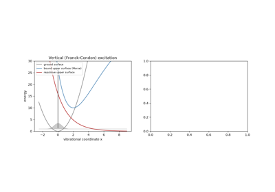
Heller’s time-dependent spectroscopy: absorption bands from short-time dynamics
1984 – Herman and Kluk’s Frozen Gaussians#
Michael Herman and Edward Kluk proposed replacing the single classical trajectory of Van Vleck theory with an entire phase-space family: launch one fixed-width (“frozen”) Gaussian wavepacket from every point of a phase-space grid, propagate each one along its own classical trajectory, and sum the results with a monodromy-built prefactor and classical action phase. Unlike a single semiclassical trajectory, this multi-trajectory (“initial value representation”) sum needs no troublesome root-finding to connect fixed endpoints, generalizes cleanly to many degrees of freedom, and – for any potential at most quadratic in position – is exact.
Implementation: physicskit.semiclassical.core.propagators.herman_kluk_propagate_wavepacket()
sums exactly such a grid of Numba-compiled classical trajectories,
built from frozen_gaussian_1d()
and herman_kluk_prefactor().
References: M. F. Herman and E. Kluk, “A Semiclassical Justification for the Use of Non-Spreading Wavepackets in Dynamics Calculations,” Chem. Phys. 91, 27-34 (1984).
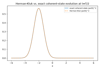
Herman-Kluk frozen-Gaussian wavepacket propagation
1984 – Heller’s Discovery of Quantum Scars#
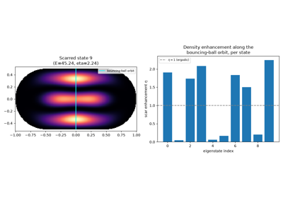
Eric Heller, numerically diagonalizing the Bunimovich stadium billiard – a paradigm chaotic system – found that a small fraction of its eigenstates were not the featureless, ergodically-spread blobs that random-matrix universality had led theorists to expect: instead they showed a clear, robust enhancement of probability density along the path of one particular unstable classical periodic orbit. These “scars” are not a violation of quantum ergodicity (which holds for almost every eigenstate as \(\hbar\to0\)) but a finite-\(\hbar\) imprint of the same periodic orbits that weight the Gutzwiller trace formula’s sum – a direct, visible link between individual eigenstates and classical chaos.
Implementation: physicskit.semiclassical.systems.scarring.bouncing_ball_energies()
and bouncing_ball_orbit_points()
concern the stadium billiard’s most famous scarred family;
scar_enhancement()
quantifies the effect directly in position space, and
husimi_projection_1d()
gives the phase-space (Husimi) view Heller himself used to first see it.
References: E. J. Heller, “Bound-State Eigenfunctions of Classically Chaotic Hamiltonian Systems: Scars of Periodic Orbits,” Phys. Rev. Lett. 53, 1515-1518 (1984).
1992 – Bogomolny’s Transfer Operator#
The Gutzwiller trace formula needs every periodic orbit, and in a chaotic system their number grows exponentially with length. Eugene Bogomolny moved the problem onto a Poincare surface of section. His transfer operator \(T(q,q';E)\) is the semiclassical propagator from one crossing of the section to the next, built from the action and stability of the short orbit segment connecting them; the levels are the zeros of \(\det[1-T(E)]\). Expanding the determinant in traces of powers of \(T\) gives back the periodic orbits as products of short segments, but the determinant itself needs only a finite matrix whose size is set by the number of wavelengths across the section. For a billiard the boundary is a natural section and \(T\) is built from chords, which makes the operator a semiclassical counterpart of the boundary-integral method.
Implementation: physicskit.semiclassical.core.bogomolny.bogomolny_transfer_operator()
builds \(T(k)\) on the boundary of a convex billiard, and
bogomolny_quantization_function()
locates its levels as the minima of the smallest singular value of
\(1-T(k)\); it reproduces the Bessel-zero spectrum of the disk and the
finite-difference spectrum of the chaotic stadium.
References: E. B. Bogomolny, “Semiclassical Quantization of Multidimensional Systems,” Nonlinearity 5, 805-866 (1992).
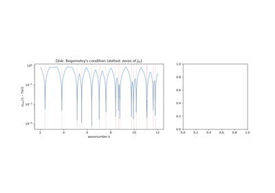
Bogomolny’s transfer operator: quantizing a billiard on its boundary