
Breakthroughs in Statistical Mechanics#
“The true logic of this world is the calculus of probabilities.” – James Clerk Maxwell, letter to Lewis Campbell, 1850
Statistical mechanics is the discovery that the definite laws of
thermodynamics – entropy, temperature, irreversibility – are nothing
but the overwhelmingly probable behavior of vast numbers of
microscopic degrees of freedom obeying ordinary, reversible mechanics.
physicskit.statphys follows that idea from a single urn of
balls to a self-organizing pile of sand, spanning lattice magnets,
disordered fluids, and critical phenomena along the way. This
chronology traces the major conceptual breakthroughs behind the
package, with a pointer to the corresponding implementation at each
stop.
1860 – Maxwell’s Distribution of Molecular Velocities#
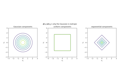
James Clerk Maxwell derived the first genuinely statistical law in physics: from little more than the isotropy of velocity space and the statistical independence of a molecule’s three velocity components, he found that a gas in equilibrium has a definite, universal distribution of molecular speeds,
extracted without ever solving an individual molecule’s equation of motion. It was, at the time, a special-case result – Maxwell assumed the distribution’s form and showed it was self-consistent under elastic collisions, for a gas already at equilibrium. Twelve years later Boltzmann would generalize the argument to interacting gases away from equilibrium and, with the H-theorem below, prove that essentially any initial velocity distribution relaxes toward exactly this Maxwellian form – turning Maxwell’s static equilibrium law into the attracting fixed point of a genuine dynamical process.
Implementation: physicskit.statphys.utils.thermodynamics.maxwell_boltzmann_speed_pdf()
evaluates exactly this equilibrium speed density in 1, 2, or 3
dimensions, and
physicskit.statphys.visualizers.particle_render.plot_velocity_histogram()
overlays it directly against the simulated speed histogram of a real
molecular dynamics trajectory.
References: J. C. Maxwell, “Illustrations of the Dynamical Theory of Gases,” Phil. Mag. Ser. 4, 19, 19-32, and 20, 21-37 (1860); L. Boltzmann, “Weitere Studien über das Wärmegleichgewicht unter Gasmolekülen,” Wiener Berichte 66, 275-370 (1872).
1870s – Boltzmann’s Statistical Entropy#
Ludwig Boltzmann proposed that a macroscopic system’s entropy simply counts the number of microscopic arrangements consistent with its observed macrostate,
an equation so central to statistical mechanics that Max Planck later had it carved on Boltzmann’s tombstone (Boltzmann himself never wrote it in exactly this form; Planck introduced the constant \(k_B\) and this notation around 1900). Boltzmann’s companion H-theorem showed that a quantity built from the single-particle velocity distribution, \(H = \int f\ln f\,d^3v\), decreases monotonically under molecular collisions – a microscopic derivation of the second law that provoked serious objections over the following decades, though not all at once: Loschmidt’s reversibility paradox arrived in 1876, just four years later, while Zermelo’s recurrence paradox followed only in 1896, nearly a quarter century on, both asking how irreversibility could possibly emerge from reversible, recurrent mechanics.
Implementation: physicskit.statphys.chapters.ehrenfest_urn.EhrenfestUrn.entropy()
computes \(S/k_B = \ln W\) exactly, via the log-gamma binomial
coefficient of the current macrostate; and
physicskit.statphys.chapters.molecular_dynamics.LennardJonesGas.h_function()
tracks Boltzmann’s H-function directly through a real molecular
dynamics trajectory, watching it decrease as the gas relaxes toward
equilibrium.
References: L. Boltzmann, “Weitere Studien über das Wärmegleichgewicht unter Gasmolekülen,” Wiener Berichte 66, 275-370 (1872); L. Boltzmann, “Über die Beziehung zwischen dem zweiten Hauptsatze der mechanischen Wärmetheorie und der Wahrscheinlichkeitsrechnung,” Wiener Berichte 76, 373-435 (1877); M. Planck, Ann. Phys. 4, 553-563 (1901).
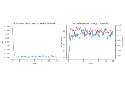
Boltzmann’s H-theorem: relaxation to the Maxwell-Boltzmann distribution
1902 – Gibbs’s Ensemble Formalism#
Josiah Willard Gibbs organized statistical mechanics around the ensemble: not a single system’s trajectory, but a probability distribution over all systems consistent with fixed macroscopic constraints – microcanonical (fixed energy), canonical (fixed temperature), and grand canonical (fixed chemical potential). Gibbs’s canonical ensemble is the workhorse of the entire field: it is what makes a Monte Carlo sampler at fixed temperature meaningful, and it ties macroscopic response functions directly to microscopic fluctuations,
These are often loosely called “fluctuation-dissipation relations,” but they are equilibrium canonical-ensemble identities – static snapshots of a system’s own thermal fluctuations – rather than the actual (dynamical) fluctuation-dissipation theorem of Callen and Welton, which relates a system’s spontaneous equilibrium fluctuations to its time-dependent linear response to an external perturbation.
Implementation: physicskit.statphys.utils.thermodynamics.specific_heat()
and susceptibility()
compute exactly these canonical-ensemble relations from a sampled
trajectory, used throughout the package – e.g. by
physicskit.statphys.chapters.ising_lattice.Ising2D.run_temperature_sweep().
References: J. W. Gibbs, Elementary Principles in Statistical Mechanics (Charles Scribner’s Sons / Yale University Press, 1902). Cf. H. B. Callen and T. A. Welton, “Irreversibility and Generalized Noise,” Phys. Rev. 83, 34-40 (1951), for the dynamical fluctuation-dissipation theorem proper.
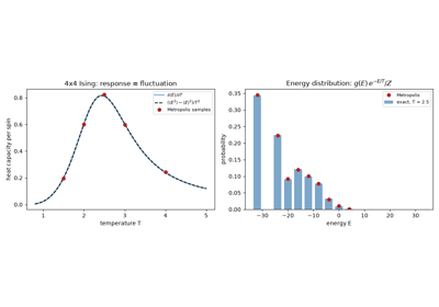
Gibbs’s canonical ensemble: response from fluctuations
1905 – Einstein’s Explanation of Brownian Motion#
Albert Einstein showed that the erratic jiggling of a pollen grain suspended in water, observed by Robert Brown in 1827, is the visible signature of unseen molecular collisions: a particle undergoing a random walk of microscopic kicks has a mean squared displacement growing linearly in time,
with diffusion coefficient \(D = k_B T / (6\pi\eta r)\) (the Stokes-Einstein relation) fixed by the fluid’s viscosity and the particle’s radius. This gave Jean Perrin an experimental handle, realized within a few years, to measure Avogadro’s number from microscope observations alone – turning “atoms” from a convenient hypothesis into a directly, quantitatively measured fact. (Coincidentally, that same year Karl Pearson posed “the problem of the random walk” in a letter to Nature, giving the underlying process its now-standard name.)
Implementation: physicskit.statphys.chapters.random_walk.RandomWalk
simulates exactly this process (lattice or continuous Gaussian steps);
mean_squared_displacement()
and diffusion_coefficient()
recover the linear-in-time law and the diffusion coefficient directly
from simulated trajectories. physicskit.statphys.chapters.langevin.BrownianMotion
integrates the overdamped Langevin equation for driven and trapped
particles, and its
measured_diffusion_coefficient()
and measured_mobility()
test the Einstein relation \(D = \mu k_B T\) itself: the spread of
the particles against their drift under a force.
stokes_einstein_diffusion_coefficient()
gives Perrin’s \(k_BT/6\pi\eta a\).
References: A. Einstein, Ann. Phys. 322(8), 549-560 (1905); K. Pearson, Nature 72, 294 (1905); J. Perrin, Ann. Chim. Phys. 18, 5-114 (1909).
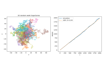
Diffusion, the Einstein relation, and the central limit theorem
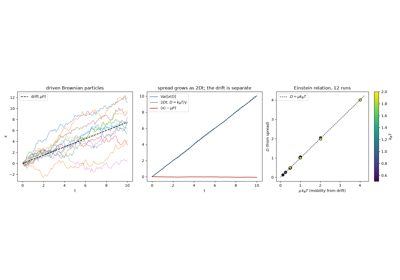
Einstein’s Brownian motion: diffusion equals mobility times temperature
1907 – The Ehrenfest Urn Model#
Paul and Tatiana Ehrenfest answered Loschmidt’s and Zermelo’s objections to Boltzmann’s H-theorem with the simplest model that could possibly settle the argument: \(N\) labeled balls split between two boxes, one ball moved at random each step. The dynamics is exactly reversible and does, in principle, recur exactly to its initial state (as Zermelo’s Poincare-recurrence objection demands) – yet for any macroscopic \(N\) the expected recurrence time is astronomically larger than the age of the universe, while the approach to the near-equal-occupancy equilibrium is essentially immediate. Reversible microphysics and an observed thermodynamic arrow of time turn out to be perfectly compatible; only the timescales involved are utterly different.
Implementation: physicskit.statphys.chapters.ehrenfest_urn.EhrenfestUrn,
step(),
and run()
reproduce exactly this reversible random-exchange dynamics and its
rapid, statistical relaxation.
References: P. Ehrenfest and T. Ehrenfest, Phys. Z. 8, 311-314 (1907).
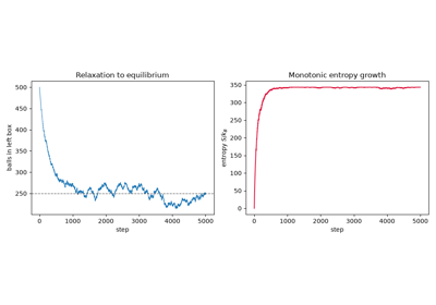
The Ehrenfest urn: reversibility, recurrence, and the arrow of time
1908 – The Langevin Equation#
Paul Langevin gave Einstein’s statistical account of Brownian motion a dynamical companion: instead of a diffusion equation for the probability of finding a particle somewhere, write Newton’s second law for the particle itself, split its interaction with the fluid into a systematic drag and a rapidly fluctuating random force,
with the noise strength fixed, by the fluctuation-dissipation balance implicit in this equation, to the same friction coefficient \(\gamma\) that damps the systematic motion. Overdamped and integrated, the Langevin equation reproduces exactly Einstein’s \(\langle x^2\rangle = 2Dt\) law and its diffusion coefficient, but it does something Einstein’s diffusion-equation picture cannot: it generates individual, simulatable stochastic trajectories, one random force realization at a time. That trajectory-level stochastic differential equation is the direct ancestor of essentially all modern stochastic simulation, including the driven, far-from-equilibrium protocols behind the Jarzynski equality below.
Implementation: physicskit.statphys.chapters.nonequilibrium_work.JarzynskiHarmonicTrap.run_protocol()
integrates exactly the overdamped Langevin equation (via
Euler-Maruyama) for a Brownian particle in a moving harmonic trap,
generating individual stochastic trajectories under a systematic drag
and a Gaussian random force of the prescribed
fluctuation-dissipation-balanced strength.
physicskit.statphys.chapters.langevin.LangevinDynamics keeps the
inertia: it integrates the full equation for particles in a harmonic trap
with the BAOAB splitting
(physicskit.integrators.stochastic.baoab_integrate()), which holds
the bath temperature for any friction, while the shared
physicskit.integrators.stochastic.euler_maruyama_integrate()
integrates any variant with a noise strength of your choosing.
References: P. Langevin, “Sur la théorie du mouvement brownien,” C. R. Acad. Sci. 146, 530-533 (1908); B. Leimkuhler and C. Matthews, “Rational construction of stochastic numerical methods for molecular sampling,” Appl. Math. Res. Express 2013, 34-56 (2013).
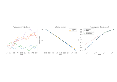
The Langevin equation: Brownian motion one trajectory at a time
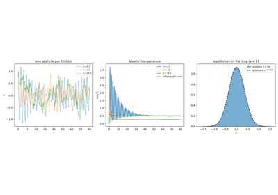
The Langevin equation: friction and noise must balance
1914-1917 – The Fokker-Planck Equation#
Adriaan Fokker, in his 1913 Leiden thesis on the Brownian motion of dipoles in a radiation field (published 1914), and Max Planck in 1917 turned Langevin’s picture around. Instead of following one random path, they wrote a deterministic equation for the probability density of all paths,
with the drift \(A\) and diffusion \(D\) read off from the Langevin equation. Its zero-flux stationary state for a particle in a potential is the Boltzmann distribution, so the equation connects Langevin’s trajectories to Gibbs’s ensembles. Kolmogorov (1931) derived the same “forward equation” for general Markov diffusions, and Kramers (1940) used it to compute the rate at which thermal noise carries a particle over an energy barrier.
Implementation: physicskit.statphys.utils.fokker_planck.fokker_planck_1d()
solves the 1D equation with a mass-conserving finite-volume
discretization, reflecting walls, and Crank-Nicolson time stepping, and
fokker_planck_stationary()
gives the closed-form zero-flux stationary density.
References: A. D. Fokker, “Die mittlere Energie rotierender elektrischer Dipole im Strahlungsfeld,” Ann. Phys. 348, 810-820 (1914); M. Planck, “Über einen Satz der statistischen Dynamik und seine Erweiterung in der Quantentheorie,” Sitzungsber. Preuss. Akad. Wiss., 324-341 (1917); H. A. Kramers, Physica 7, 284-304 (1940); H. Risken, The Fokker-Planck Equation, 2nd ed. (Springer, 1989).
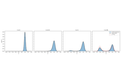
The Fokker-Planck equation: from noisy trajectories to a deterministic density
1920-1925 – The Ising Model#
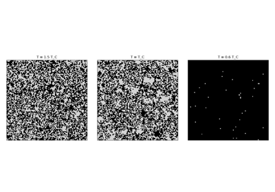
Wilhelm Lenz proposed, and his student Ernst Ising solved (in his 1924 doctoral thesis, published in 1925), the simplest possible model of a magnet: spins \(s_i = \pm 1\) on a lattice, coupled to their nearest neighbors, with Hamiltonian \(H = -J\sum_{\langle i,j\rangle} s_i s_j\). Ising’s exact one-dimensional solution found no phase transition at any nonzero temperature – a disappointing result he (incorrectly) suspected would hold in every dimension, very nearly burying the model before it had a chance to prove its worth. In two and more dimensions, as would only be settled two decades later, the model does order ferromagnetically below a critical temperature, and it has since become the single most-studied model in statistical mechanics: a minimal system exhibiting a genuine continuous phase transition, spontaneous symmetry breaking, and (as later understood) universal critical behavior shared with wildly different physical systems.
References: W. Lenz, Phys. Z. 21, 613-615 (1920); E. Ising, “Beitrag zur Theorie des Ferromagnetismus,” Z. Phys. 31, 253-258 (1925).
1924-1926 – Bose-Einstein and Fermi-Dirac Quantum Statistics#
Satyendra Nath Bose’s 1924 rederivation of Planck’s radiation law – by treating photons as indistinguishable, unlabeled particles counted purely by how many occupy each state, rather than as classically labeled objects – caught Einstein’s attention enough that he translated it, extended it to massive particles, and predicted something Bose had not: below a critical temperature, a macroscopic fraction of the particles collapses into the single-particle ground state, a new phase of matter with no classical analogue. This Bose-Einstein condensation (BEC) was not observed directly until 1995, in dilute alkali-atom gases cooled to nanokelvin temperatures (Cornell and Wieman; Ketterle independently; 2001 Nobel Prize). Enrico Fermi and Paul Dirac found, independently and almost simultaneously (1926, though Fermi’s paper was received some six months before Dirac’s), the complementary statistics obeyed by indistinguishable particles subject to the Pauli exclusion principle: no state may ever hold more than one such particle, which sharpens into a hard Fermi surface at \(T=0\) and underlies the stability of ordinary matter, the behavior of metals, and the structure of white dwarfs and neutron stars.
both of which reduce to the classical Maxwell-Boltzmann distribution \(n \approx e^{-(\varepsilon-\mu)/k_B T}\) when occupation numbers are small (\(\varepsilon - \mu \gg k_B T\)). For a homogeneous ideal Bose gas, the condensate fraction below \(T_c\) follows
Implementation: physicskit.statphys.utils.thermodynamics.bose_einstein_occupation()
and fermi_dirac_occupation()
compute the two quantum occupation numbers directly;
bec_condensate_fraction()
reproduces the ideal-gas condensate curve confirmed in the 1995 experiments,
and maxwell_boltzmann_speed_pdf()
gives the classical high-temperature limit both quantum distributions
converge to.
References: S. N. Bose, Z. Phys. 26, 178-181 (1924); A. Einstein, Sitzungsber. Preuss. Akad. Wiss., 261-267 (1924), and 3-14 (1925); E. Fermi, Rend. Lincei 3, 145-149 (1926); P. A. M. Dirac, Proc. R. Soc. A 112, 661-677 (1926); M. H. Anderson et al., Science 269, 198-201 (1995); K. B. Davis et al., Phys. Rev. Lett. 75, 3969-3973 (1995).
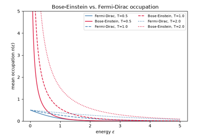
Quantum statistics: Bose-Einstein, Fermi-Dirac, and condensation
1930 – The Ornstein-Uhlenbeck Process#
George Uhlenbeck and Leonard Ornstein solved Langevin’s equation exactly for the velocity of a free Brownian particle, and found that it is not white noise but a process with memory,
The velocity forgets its initial value on the time scale \(1/\theta = m/\gamma\) and settles to the stationary variance \(\sigma^2/2\theta = k_BT/m\), while the position diffuses ballistically at short times and with Einstein’s \(2Dt\) at long times. Doob (1942) proved it is the only process that is stationary, Gaussian, and Markov at once, which is why it reappears as the model of any linearly restored noisy variable: a particle in an optical trap, a thermally agitated circuit, an interest rate.
Implementation: physicskit.statphys.chapters.langevin.OrnsteinUhlenbeck
samples ensembles of paths with the exact Gaussian transition or by
Euler-Maruyama integration, and provides the closed-form mean, variance,
and stationary autocovariance they are checked against.
References: G. E. Uhlenbeck and L. S. Ornstein, “On the theory of the Brownian motion,” Phys. Rev. 36, 823-841 (1930); J. L. Doob, “The Brownian movement and stochastic equations,” Ann. Math. 43, 351-369 (1942).
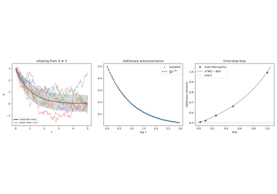
The Ornstein-Uhlenbeck process: Gaussian noise with a memory
1937 – Landau Mean-Field Theory#
Rather than derive a phase transition from a microscopic Hamiltonian, Lev Landau asked what the free energy itself must look like near a continuous transition, given only the symmetry of an order parameter \(m\) that the disordered phase forbids from appearing at odd powers. The simplest possible expansion consistent with that symmetry,
reproduces, from analyticity and symmetry alone, the qualitative shape of every continuous transition: a single minimum at \(m=0\) above \(T_C\), a spontaneously broken pair of minima below it, and a susceptibility diverging on both sides. Landau theory’s mean-field critical exponents (\(\beta = 1/2\), \(\gamma = 1\)) are quantitatively wrong in low dimensions – Onsager’s exact solution below gives \(\beta = 1/8\) in two dimensions instead – a discrepancy the renormalization group would not fully explain for another three decades. But the qualitative order-parameter picture Landau introduced, and the idea of classifying transitions by how they break symmetry, underlies the entire modern theory of phase transitions built on top of it.
Implementation: physicskit.statphys.utils.landau_theory.landau_free_energy()
evaluates \(F(m,T)\) directly;
landau_equilibrium_magnetization()
finds its minimizing \(m(T)\), reproducing the mean-field
\(\beta=1/2\) power law, and
landau_susceptibility()
gives the diverging zero-field susceptibility on both sides of \(T_C\).
The same minimizer, with nonzero h, also traces the field-driven
\(m(h)\) response at fixed \(T\), showing the globally stable
branch responding smoothly above \(T_C\) but jumping discontinuously
through \(h=0\) below it.
References: L. Landau, Zh. Eksp. Teor. Fiz. 7, 19-32, and 627-632 (1937).
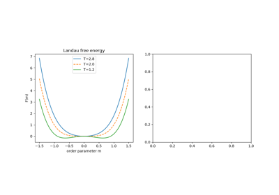
Landau mean-field theory: order parameters from symmetry alone
1944 – Onsager’s Exact Solution of the 2D Ising Model#
Lars Onsager achieved what many considered impossible: an exact, closed-form solution of the two-dimensional Ising model in zero field, computing its free energy and locating a genuine second-order phase transition at
Onsager’s solution remains one of the few exactly solved interacting models in statistical mechanics, and the definitive proof that Ising’s pessimistic one-dimensional intuition does not generalize: dimension matters enormously to whether a phase transition can occur at all.
Implementation: physicskit.statphys.chapters.ising_lattice.Ising2D
implements the model with both single-spin Metropolis and Wolff-cluster
dynamics; its
T_C property
is Onsager’s exact critical temperature, reproduced to machine
precision from the closed-form expression above.
References: L. Onsager, “Crystal Statistics. I. A Two-Dimensional Model with an Order-Disorder Transition,” Phys. Rev. 65, 117-149 (1944).
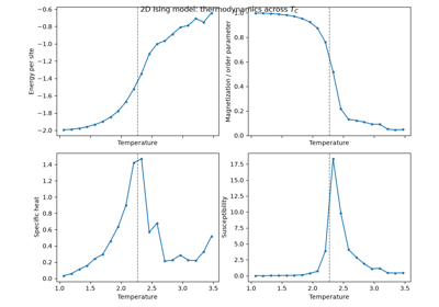
Onsager’s exact solution: the 2D Ising phase transition
1944-1955 – Itô’s Stochastic Calculus and the Euler-Maruyama Scheme#
Langevin’s white-noise force has no ordinary meaning: Brownian paths are nowhere differentiable. Kiyosi Itô (1944) defined integrals against Brownian motion directly and built a calculus for them in which \(dW^2 = dt\), so that a function of a diffusing variable picks up an extra drift \(\tfrac12 f''\,b^2\). Gisiro Maruyama (1955) showed that the obvious time-stepping of an Itô equation, \(X_{n+1} = X_n + a\,\Delta t + b\,\Delta W_n\), converges to its solution. Path by path, though, the error only shrinks as \(\Delta t^{1/2}\). Grigori Milstein (1974) added the next term of Itô’s expansion, \(\tfrac12 b b'(\Delta W^2 - \Delta t)\), and raised the order to 1. These schemes are what “simulating a Langevin equation” means in practice.
Implementation: physicskit.integrators.stochastic.euler_maruyama_integrate()
and milstein_integrate() integrate
diagonal-noise Itô equations with the package-wide
f(state, t, params) callback convention, driven by caller-supplied
Wiener increments from
wiener_increments() so that one
Brownian path can be replayed at several step sizes.
References: K. Itô, “Stochastic integral,” Proc. Imp. Acad. Tokyo 20, 519-524 (1944); G. Maruyama, “Continuous Markov processes and stochastic equations,” Rend. Circ. Mat. Palermo 4, 48-90 (1955); G. N. Milstein, Theory Probab. Appl. 19, 557-562 (1974); P. E. Kloeden and E. Platen, Numerical Solution of Stochastic Differential Equations (Springer, 1992).
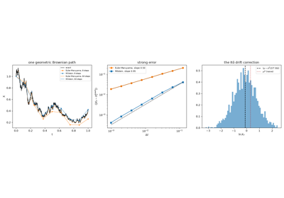
Itô’s stochastic calculus: the Euler-Maruyama and Milstein schemes
1952 – The Yang-Lee Circle Theorem#
A finite system’s partition function is a finite sum of manifestly analytic terms – so where can a genuine phase transition, a true discontinuity in the free energy, possibly come from? Tsung-Dao Lee and Chen-Ning Yang’s answer was to continue the partition function into the complex fugacity plane and study its zeros. Writing the Ising Hamiltonian with an external field, \(H = -J\sum_{\langle i,j \rangle} s_i s_j - h \sum_i s_i\), and the fugacity \(z = e^{2\beta h}\), the partition function is (up to a nonvanishing analytic prefactor) a degree-\(N\) polynomial in \(z\). Lee and Yang proved that for a ferromagnetic system, every one of that polynomial’s zeros lies exactly on the unit circle,
no matter the system size – and that a phase transition occurs, in the \(N \to \infty\) limit, exactly where these zeros pinch the positive real axis at \(z=1\) (\(h=0\)). This gave the field its first rigorous, model-independent picture of why a phase transition is mathematically possible at all, despite every finite-system ingredient being perfectly smooth.
Implementation: physicskit.statphys.utils.partition_function.ising_partition_polynomial()
enumerates a small Ising chain’s \(2^N\) configurations exactly and
returns \(Z\) as a polynomial in the fugacity, and
yang_lee_zeros() finds
that polynomial’s roots directly, reproducing the exact unit circle to
machine precision for any ferromagnetic coupling.
References: C. N. Yang and T. D. Lee, “Statistical Theory of Equations of State and Phase Transitions. I. Theory of Condensation,” Phys. Rev. 87, 404-409 (1952); T. D. Lee and C. N. Yang, “Statistical Theory of Equations of State and Phase Transitions. II. Lattice Gas and Ising Model,” Phys. Rev. 87, 410-419 (1952).
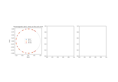
The Lee-Yang circle theorem: partition function zeros in the complex plane
1952 – The Potts Model#
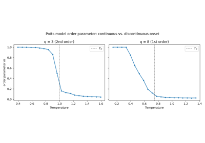
Renfrey Potts, in his 1951 Cambridge doctoral thesis (published 1952, building on a suggestion by his advisor Cyril Domb), generalized Ising’s two-state spin to \(q\) discrete states, rewarding neighboring sites only for matching exactly rather than for a continuous degree of alignment. This single generalization organizes an entire family of transitions within one model: \(q=2\) recovers the Ising model exactly (with a rescaled coupling), while on the square lattice the transition sharpens from continuous (second order) at \(q \le 4\) to discontinuous (first order) at \(q > 4\) – making the Potts model the cleanest available laboratory for watching a phase transition’s order itself change as a single parameter is dialed. Its random-cluster (Fortuin-Kasteleyn) representation later became a bridge connecting statistical mechanics to graph theory and the Tutte polynomial.
Implementation: physicskit.statphys.chapters.ising_lattice.PottsModel2D
implements exactly this q-state generalization; its
T_C property
gives the exact square-lattice critical temperature
\(J/(k_B \ln(1+\sqrt q))\), and
order_parameter()
tracks the rescaled majority-state fraction whose transition sharpens from
continuous to discontinuous as \(q\) increases past 4.
References: R. B. Potts, Proc. Cambridge Phil. Soc. 48, 106-109 (1952).
First- versus second-order transitions in the q-state Potts model
1953 – The Metropolis Algorithm#
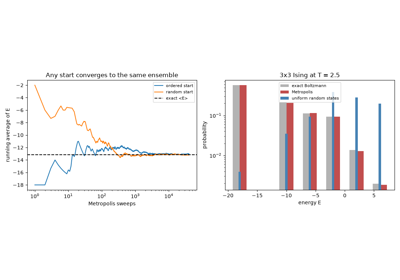
Nicholas Metropolis, Arianna and Marshall Rosenbluth, and Augusta and Edward Teller introduced a way to sample a canonical (Gibbs) ensemble without ever computing its normalizing partition function: propose a random local change, and accept it with probability \(\min(1, e^{-\beta\Delta E})\). Iterated, this Markov chain converges to exactly the Boltzmann-weighted equilibrium distribution – and turned statistical mechanics from a field of exactly solvable special cases (like Onsager’s) into one where almost any model could be simulated on a computer. It remains, seventy years later, the algorithm underneath essentially every Monte Carlo statistical-mechanics calculation, including every lattice-model chapter in this package.
Implementation: physicskit.statphys.core.monte_carlo.metropolis_sweep_ising()
and its counterparts
metropolis_sweep_potts(),
metropolis_sweep_xy(), and
metropolis_sweep_spin_glass()
are the Numba-JIT-compiled Metropolis-Hastings kernels driving every
lattice-model chapter (Ising2D,
PottsModel2D,
XYModel2D,
EdwardsAndersonSpinGlass2D)
in the package.
References: N. Metropolis, A. W. Rosenbluth, M. N. Rosenbluth, A. H. Teller, and E. Teller, “Equation of State Calculations by Fast Computing Machines,” J. Chem. Phys. 21, 1087-1092 (1953).
The Metropolis algorithm: sampling Boltzmann without the partition function
1957 – Molecular Dynamics Simulation#
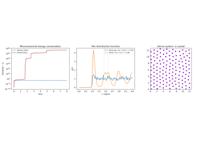
Berni Alder and Thomas Wainwright took a different route to the same goal: rather than sampling configurations stochastically, integrate Newton’s equations for hundreds of interacting hard-sphere particles directly, and let equilibrium statistics emerge from the trajectory itself. Their 1957 discovery of a fluid-solid phase transition in a system of pure hard spheres, with no attractive interaction at all, was itself a landmark: order could arise from packing constraints alone. Molecular dynamics – generalized to continuous potentials like the Lennard-Jones interaction, and put on a firm symplectic footing with integrators such as Velocity Verlet – remains the direct-simulation complement to Metropolis-style Monte Carlo throughout physics, chemistry, and biology.
Implementation: physicskit.statphys.chapters.molecular_dynamics.LennardJonesGas
integrates exactly this kind of system via
physicskit.statphys.core.md_engine.lj_forces() and
velocity_verlet_step(),
letting an arbitrary non-equilibrium initial velocity distribution
relax toward the Maxwell-Boltzmann form under real Newtonian dynamics.
References: B. J. Alder and T. E. Wainwright, J. Chem. Phys. 27, 1208-1209 (1957).
Alder and Wainwright: molecular dynamics simulation
1957 – Percolation Theory#
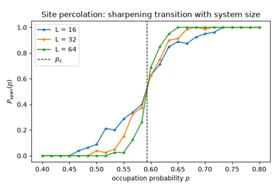
Simon Broadbent and John Hammersley introduced percolation theory to model fluid flow through a random porous medium: occupy each site (or bond) of a lattice independently with probability \(p\), and ask whether a connected path spans the system. Below a sharp threshold \(p_c\) only finite clusters exist; above it, an infinite spanning cluster appears with probability one. Unlike a thermal phase transition, percolation has no energy scale or temperature at all – the transition is purely geometric – yet it displays the full apparatus of critical phenomena: a sharp threshold, power-law cluster-size distributions, and universal critical exponents, making it the cleanest possible laboratory for studying criticality itself.
Implementation: physicskit.statphys.chapters.percolation.Percolation2D
generates site and bond percolation configurations and labels their
clusters via hoshen_kopelman();
its p_c
property gives the known square-lattice thresholds (\(p_c \approx
0.592746\) for sites, \(p_c = 0.5\) exactly for bonds, by
self-duality).
References: S. R. Broadbent and J. M. Hammersley, Proc. Cambridge Phil. Soc. 53, 629-641 (1957).
1971 – Wilson’s Renormalization Group#
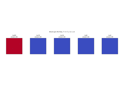
Leo Kadanoff’s 1966 block-spin picture – group a lattice into blocks, replace each block by a single effective spin, and ask how the effective coupling changes – gave universality and scaling an intuitive geometric story. Kenneth Wilson turned that picture into a rigorous calculational framework, the renormalization group, showing that repeated coarse-graining defines a flow on the space of possible Hamiltonians whose fixed points – ordered, disordered, and critical – organize all of critical phenomena, and explain why wildly different microscopic systems can share identical critical exponents (the same “universality class”). The renormalization group, for which Wilson received the 1982 Nobel Prize, is now understood as one of the deepest organizing ideas in all of theoretical physics, far beyond its statistical-mechanics origin.
Implementation: physicskit.statphys.chapters.renormalization.BlockSpinRG
implements exactly Kadanoff’s \(2\times2\) majority-rule
block-spin transformation on an Ising configuration;
coarse_grain_step()
performs one coarse-graining step and
iterate()
follows the resulting flow toward the ordered, disordered, or critical
fixed point.
References: L. P. Kadanoff, Physics 2, 263-272 (1966); K. G. Wilson, Phys. Rev. B 4, 3174-3183 (1971), and 3184-3205 (1971).
1971-1973 – Vortex Unbinding in the 2D XY Model#
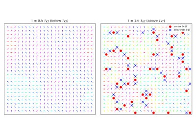
Vadim Berezinskii showed in 1971 (in an English translation of a 1970 Russian original) that the two-dimensional XY model of planar spins \(\theta_i \in [0, 2\pi)\) – forbidden by the Mermin-Wagner theorem from ever developing conventional long-range order – nonetheless undergoes a genuine phase transition, driven entirely by the unbinding of topological vortex-antivortex pairs; John Kosterlitz and David Thouless, working independently and arriving at the transition two years later, in 1973, gave the mechanism its now-standard, more complete treatment, with Kosterlitz following up in 1974 with the renormalization-group analysis of the unbinding itself. Below the transition temperature, vortices remain bound in tightly circling pairs of opposite topological charge; above it, thermal fluctuations tear these pairs apart into a free “vortex plasma,” destroying the algebraic quasi-long-range order of the low-temperature phase. Kosterlitz and Thouless shared the 2016 Nobel Prize in part for this work (Berezinskii, who died in 1980, was by then long ineligible); the transition is nonetheless routinely credited to all three names today, and is often written “BKT” in recognition of Berezinskii’s priority.
Implementation: physicskit.statphys.chapters.ising_lattice.XYModel2D
simulates exactly this lattice of planar spins; its
T_KT
property gives the numerically established transition temperature
(\(\approx 0.893\,J/k_B\)), and
vorticity()
(backed by
physicskit.statphys.core.monte_carlo.xy_plaquette_vorticity())
measures the integer topological charge of every plaquette directly,
making the bound-pair-to-plasma unbinding visible configuration by
configuration.
References: V. L. Berezinskii, Sov. Phys. JETP 32, 493-500 (1971) (English translation of the 1970 Russian original); J. M. Kosterlitz and D. J. Thouless, J. Phys. C 6, 1181-1203 (1973); J. M. Kosterlitz, J. Phys. C 7, 1046-1060 (1974).
The Kosterlitz-Thouless transition: vortex-antivortex unbinding
1975 – The Edwards-Anderson Spin Glass#
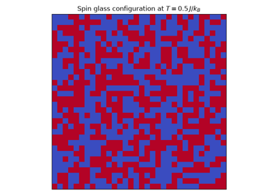
Sam Edwards and Philip Anderson proposed that magnetic alloys with random, competing ferromagnetic and antiferromagnetic interactions freeze, below a sharp temperature, into a disordered but static configuration – a “spin glass” – held together not by translational order but by the sheer geometric impossibility of satisfying every bond at once. A plaquette with an odd number of antiferromagnetic bonds is frustrated: no single spin configuration minimizes all of its bonds simultaneously, and the resulting ground state is highly degenerate, dominated by a rugged hierarchy of nearly-equal-energy valleys rather than one clean minimum. Detecting the transition demanded a genuinely new order parameter, since the ordinary magnetization stays zero on both sides of it: Edwards and Anderson compared two independently thermalized replicas subject to the same quenched disorder, whose spin overlap freezes to a nonzero value below the spin-glass transition and decorrelates to zero above it.
Implementation: physicskit.statphys.chapters.spin_glass.EdwardsAndersonSpinGlass2D
implements exactly this \(\pm J\) bimodal-disorder Ising spin glass;
frustration_density()
measures the fixed, geometric fraction of frustrated plaquettes, and
edwards_anderson_order_parameter()
estimates \(\langle q^2 \rangle\) from two independently thermalized
replicas sharing the same bonds.
References: S. F. Edwards and P. W. Anderson, J. Phys. F 5, 965-974 (1975).
Spin glasses: frustration and the Edwards-Anderson order parameter
1975-1980 – The Sherrington-Kirkpatrick Model and Parisi’s Replica Symmetry Breaking#
The same year as Edwards and Anderson’s short-range model, David Sherrington and Scott Kirkpatrick proposed the opposite extreme: every spin coupled to every other spin, with independent Gaussian bonds,
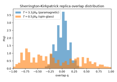
Its infinite-range connectivity made the model look exactly solvable by the replica trick – until the naive replica-symmetric ansatz produced a manifestly unphysical negative entropy at low temperature, a glaring sign that something in the calculation was wrong. Giorgio Parisi’s 1979-1980 resolution was to break replica symmetry itself: rather than one frozen ground state, the low-temperature phase is an infinite, hierarchically nested family of pure states, organized by a nontrivial, sample-dependent distribution \(P(q)\) of the replica overlap
rather than the single frozen value the Edwards-Anderson picture predicts. Parisi’s replica-symmetry-breaking solution – rigorously proven correct only decades later (Talagrand, 2006; Guerra’s bound, 2003) – earned him a share of the 2021 Nobel Prize, and its hierarchical “ultrametric” structure went on to find applications far outside physics, from neural networks and combinatorial optimization to protein folding.
Implementation: physicskit.statphys.chapters.spin_glass.SherringtonKirkpatrick
implements exactly this fully-connected Gaussian-disorder spin glass;
overlap_distribution()
pools replica-overlap samples across many independent disorder
realizations, exposing – in a finite-size Monte Carlo simulation – the
broad, non-self-averaging \(P(q)\) that is the numerically observable
fingerprint of Parisi’s replica-symmetry-breaking solution.
References: D. Sherrington and S. Kirkpatrick, Phys. Rev. Lett. 35, 1792-1796 (1975); G. Parisi, Phys. Rev. Lett. 43, 1754-1756 (1979), and J. Phys. A 13, L115-L121 (1980); F. Guerra, Commun. Math. Phys. 233, 1-12 (2003); M. Talagrand, Ann. Math. 163, 221-263 (2006).
The Sherrington-Kirkpatrick model and Parisi’s replica overlap
1979-1981 – Path-Integral Monte Carlo#
Feynman had shown in 1953 that the partition function of quantum particles is a path integral in imaginary time, and that each quantum particle then behaves like a classical closed polymer. Barker (1979) turned this into an algorithm: slice the imaginary-time interval \(\beta\hbar\) into \(P\) steps of width \(\tau = \beta/P\), and in the primitive (Trotter) approximation
a classical ring polymer of \(P\) beads joined by harmonic springs, which ordinary Metropolis moves can sample. The error is \(O(\tau^2)\), so the result becomes exact as \(P \to \infty\). Chandler and Wolynes (1981) made the quantum-classical isomorphism explicit, including the cross-linking of polymers by exchange for bosons. Ceperley’s later work on liquid helium-4, where the polymers wind around the periodic box to give a superfluid fraction, made path-integral Monte Carlo the standard exact method for bosons at finite temperature.
Implementation: physicskit.statphys.chapters.path_integral.PathIntegralParticle
samples the ring polymer of one particle in the well
\(V = \tfrac12\omega^2 x^2 + \lambda x^4\) with bead and centroid
moves, measuring \(\langle x^2 \rangle\) and the virial energy;
harmonic_x2_primitive()
gives the exact \(P\)-bead target for the harmonic case, and
harmonic_x2_exact() its
\(P \to \infty\) limit.
References: R. P. Feynman, Phys. Rev. 91, 1291-1301 (1953); J. A. Barker, J. Chem. Phys. 70, 2914-2918 (1979); D. Chandler and P. G. Wolynes, J. Chem. Phys. 74, 4078-4095 (1981); D. M. Ceperley, Rev. Mod. Phys. 67, 279-355 (1995).
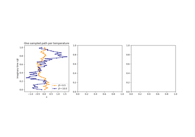
Path-integral Monte Carlo: a quantum particle as a classical ring polymer
1981 – The Binder Cumulant and Finite-Size Scaling#
Kurt Binder introduced a scale-independent diagnostic for locating a continuous phase transition from necessarily finite simulations: the fourth-order cumulant of the order parameter, dimensionless by construction, whose curves at different lattice sizes \(L\) all cross at very nearly the same point – the infinite-volume critical temperature – because at criticality \(U_4\) depends on \(L\) only through the universal combination \(L^{1/\nu}\). This turned finite-size effects, previously seen only as an inconvenient rounding of what should be a sharp singularity, into a precision tool: simulating a handful of modest lattice sizes and finding where their Binder-cumulant curves cross extracts both \(T_C\) and the critical exponents without ever having to simulate an infinite system.
Implementation: physicskit.statphys.utils.thermodynamics.binder_cumulant()
computes \(U_4\) from a magnetization sample; the
physicskit.statphys.utils.finite_size_scaling module implements the
full analysis built on it –
binder_cumulant_crossing()
locates \(T_C\) as the crossing of two lattice sizes’ \(U_4(T)\)
curves, and
estimate_gamma_over_nu(),
estimate_beta_over_nu(),
and
estimate_nu_from_binder_slope()
extract the critical exponents from the corresponding finite-size scaling
laws.
References: K. Binder, Z. Phys. B 43, 119-140 (1981).
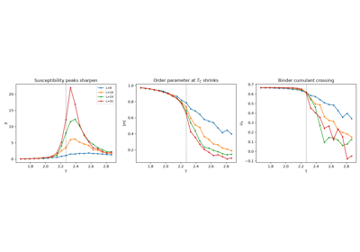
Finite-size scaling: extracting critical exponents
1986 – The Kardar-Parisi-Zhang Equation#
Mehran Kardar, Giorgio Parisi, and Yi-Cheng Zhang proposed a stochastic partial differential equation for a generic growing interface – crystal surfaces, bacterial colonies, burning paper fronts – driven by uncorrelated noise, smoothed by surface tension, and locally accelerated by growth normal to the surface rather than straight up:
That nonlinear \((\nabla h)^2\) term is what separates the KPZ universality class from the simpler, linear Edwards-Wilkinson equation (\(\lambda=0\)): it couples length scales together and forces a wholly new set of scaling exponents on the interface width \(w(t) = \sqrt{\langle(h-\bar h)^2\rangle}\), growing as \(w \sim t^\beta\) (\(\beta=1/3\) in 1+1 dimensions) before saturating at \(w_{\text{sat}} \sim L^\alpha\) (\(\alpha=1/2\)) once the system size is reached. These exponents turned out to be extraordinarily universal, appearing (both theoretically and experimentally) in systems with no obvious surface at all, from directed polymers to burning fronts, and to have deep, still-active connections to random matrix theory.
Implementation: physicskit.statphys.core.kpz_engine.run_rsos() and
physicskit.statphys.chapters.kpz_growth.KPZInterface implement
the Restricted Solid-On-Solid growth automaton, an exact discrete model
with no adjustable surface-tension or coupling constants that is long
established to lie in the KPZ universality class;
run_growth_curve()
recovers both the \(\beta=1/3\) growth exponent and the
\(\alpha=1/2\) saturation exponent directly from simulation.
References: M. Kardar, G. Parisi, and Y.-C. Zhang, Phys. Rev. Lett. 56, 889-892 (1986).
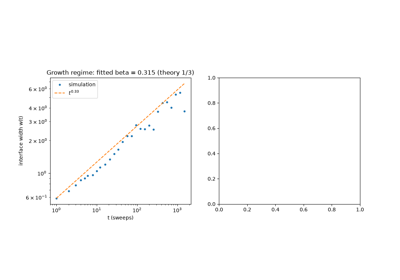
Universal interface roughening: the Kardar-Parisi-Zhang universality class
1987 – Self-Organized Criticality and the BTW Sandpile#
Per Bak, Chao Tang, and Kurt Wiesenfeld asked whether a system could reach a critical state – power-law-distributed fluctuations at every scale – without anyone fine-tuning a parameter to a special value, the way temperature must be tuned to \(T_c\) in the Ising model. Their sandpile automaton answers yes: grains added one at a time to a lattice topple whenever a site’s height exceeds a threshold, and the slow-driving, fast-relaxation dynamics tunes the pile itself to a critical state, with avalanche sizes following a power law with no characteristic scale. “Self-organized criticality” was proposed as a generic mechanism for the ubiquity of power laws in nature – earthquakes, forest fires, neural avalanches – and remains one of the most influential, and most debated, ideas to come out of statistical physics in the last fifty years.
Implementation: physicskit.statphys.chapters.sandpile.BTWSandpile
implements exactly this toppling automaton;
run() drives
the pile with a stream of randomly placed grains and records each
one’s avalanche size, backed by
physicskit.statphys.core.sandpile_engine.topple_to_stability().
Repeating this at several grid sizes and fitting the growth of the largest
observed avalanche with
power_law_exponent()
recovers the finite-size cutoff’s own scaling with \(L\).
References: P. Bak, C. Tang, and K. Wiesenfeld, Phys. Rev. Lett. 59, 381-384 (1987).
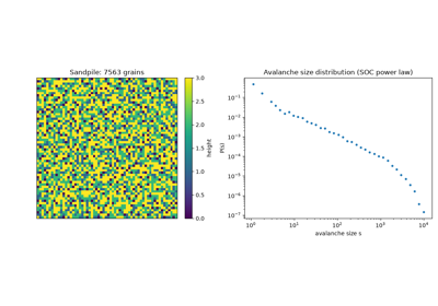
Self-organized criticality: the Bak-Tang-Wiesenfeld sandpile
1987 – The Swendsen-Wang Cluster Algorithm#
Even Metropolis dynamics suffers from critical slowing down: single-spin flips decorrelate a configuration only diffusively, so the autocorrelation time diverges as a power of the lattice size, \(\tau \sim L^z\) with \(z \approx 2.17\), exactly where accurate statistics matter most, at \(T_C\). Robert Swendsen and Jian-Sheng Wang broke this bottleneck with the first cluster algorithm. They used the Fortuin-Kasteleyn representation (1972), which writes the Ising partition function as a sum over bond configurations: every bond between two aligned neighbors is activated with probability
and, given the activated bonds, the spins of each connected cluster are free to take either sign. One Swendsen-Wang update therefore draws the bonds, labels the clusters, and flips each cluster independently with probability 1/2, resampling the whole lattice at once. Because the clusters are the physical correlated domains, the update is a global move and the dynamical exponent drops to \(z \approx 0.2\). The same idea carries over to the Potts model and, through embedding, to continuous spins.
Implementation: physicskit.statphys.core.monte_carlo.swendsen_wang_step_ising()
activates the bonds, labels the clusters with union-find and flips each
with probability 1/2; it backs
physicskit.statphys.chapters.ising_lattice.Ising2D.sweep()
(algorithm="swendsen-wang").
References: C. M. Fortuin and P. W. Kasteleyn, Physica 57, 536-564 (1972); R. H. Swendsen and J.-S. Wang, Phys. Rev. Lett. 58, 86-88 (1987).
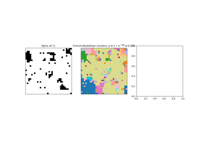
The Swendsen-Wang algorithm: flipping every Fortuin-Kasteleyn cluster at once
1989 – The Wolff Cluster Algorithm#
Swendsen and Wang’s update partitions the whole lattice into clusters, including many small ones whose flips barely change anything. Ulli Wolff’s 1989 refinement grows and flips just one cluster per update, seeded at a random site, with each bond added independently with probability \(p_{\text{add}} = 1 - e^{-2\beta J}\). A random site is more likely to lie in a large cluster, so the moves Wolff makes are, on average, the large correlated domains that matter; the algorithm’s dynamical critical exponent is dramatically smaller than Metropolis’s, turning simulations right at \(T_C\) – previously the hardest regime to sample – into one of the easiest.
Implementation: physicskit.statphys.core.monte_carlo.wolff_step_ising()
implements exactly this cluster growth and flip, and backs
physicskit.statphys.chapters.ising_lattice.Ising2D.sweep()
(algorithm="wolff"); it is also what
BlockSpinRG uses to
equilibrate its initial fine-grained configuration reliably even deep below
\(T_C\), where single-spin Metropolis dynamics would stall on slow
domain-wall coarsening.
References: R. H. Swendsen and J.-S. Wang, Phys. Rev. Lett. 58, 86-88 (1987); U. Wolff, Phys. Rev. Lett. 62, 361-364 (1989).
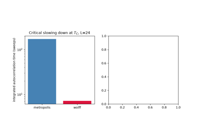
The Wolff cluster algorithm: beating critical slowing down
1997 – The Jarzynski Equality#
The second law only bounds the average work needed to drive a system between two equilibrium states, \(\langle W \rangle \ge \Delta F\), with equality only in the reversible, infinitely slow limit – any individual fast, irreversible realization tells you nothing exact about \(\Delta F\) on its own. Christopher Jarzynski found an exact equality hiding behind that inequality: averaging not \(W\) itself but \(e^{-\beta W}\) over an ensemble of repeated, arbitrarily fast realizations of the same protocol recovers the equilibrium free energy difference exactly,
no matter how far from equilibrium any individual trajectory is driven. Jensen’s inequality applied to this identity immediately reproduces the second law as a corollary rather than an independent postulate – nonequilibrium work fluctuations turn out to carry exact equilibrium information. The result kicked off modern nonequilibrium statistical mechanics, including the closely related Crooks fluctuation theorem (1999) and single-molecule “pulling” experiments that now measure protein and RNA folding free energies this way.
Implementation: physicskit.statphys.chapters.nonequilibrium_work.JarzynskiHarmonicTrap
drags a Brownian particle’s harmonic trap at finite speed via overdamped
Langevin dynamics;
jarzynski_free_energy_estimate()
recovers the exact \(\Delta F = 0\) of this translation-invariant trap
(the stiffness never changes, only its center moves) from the same
irreversible work samples whose mean, by the second law, sits strictly
above zero.
References: C. Jarzynski, Phys. Rev. Lett. 78, 2690-2693 (1997); G. E. Crooks, Phys. Rev. E 60, 2721-2726 (1999).
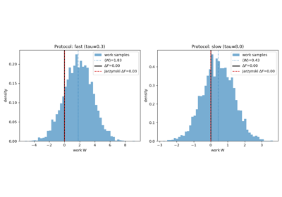
Jarzynski’s equality: exact free energies from irreversible work
2001 – Wang-Landau Flat-Histogram Sampling#
Metropolis sampling, cluster or not, works at one temperature, and a first-order transition or a rugged energy landscape traps it in one basin. Fugao Wang and David Landau proposed estimating the density of states \(g(E)\) directly instead, by a random walk in energy space. A move from \(E_1\) to \(E_2\) is accepted with probability
and after every step the estimate of the current level is raised, \(\ln g(E) \to \ln g(E) + \ln f\). The walk is thus driven away from levels it has already visited until its histogram is flat; then \(\ln f\) is halved and the walk restarts, and the estimate converges as \(\ln f \to 0\). With \(g(E)\) in hand, the partition function \(Z(\beta) = \sum_E g(E) e^{-\beta E}\), the free energy and the entropy, quantities that canonical sampling cannot give directly, follow at every temperature from one run. The method spread quickly to protein folding, liquids and quantum systems.
Implementation: physicskit.statphys.chapters.wang_landau.WangLandauIsing
runs the walk on the 2D Ising lattice (kernel
physicskit.statphys.core.monte_carlo.wang_landau_sweeps_ising());
ising_density_of_states_exact()
enumerates the exact \(g(E)\) of a \(4\times4\) lattice to check
it against, and
canonical_from_density_of_states()
turns either into canonical averages.
References: F. Wang and D. P. Landau, Phys. Rev. Lett. 86, 2050-2053 (2001); Phys. Rev. E 64, 056101 (2001).
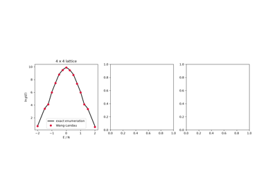
Wang-Landau sampling of the Ising density of states