
Breakthroughs in General Relativity#
“Spacetime tells matter how to move; matter tells spacetime how to curve.” – John Archibald Wheeler
General relativity replaced Newton’s instantaneous force of gravity with a
single geometric idea: mass and energy curve spacetime, and free-falling
objects simply follow the straightest paths available in that curved
geometry. From that one idea, worked out by Einstein over a decade of false
starts, followed black holes, an expanding universe, and ripples in
spacetime itself that would not be directly observed for another century.
The chronology behind physicskit.relativity traces that century, from
Einstein’s 1915 field equations to the Event Horizon Telescope’s first
image of a black hole’s shadow in 2019, with a pointer to the corresponding
implementation in this package at each stop.
1915 – Einstein’s Field Equations#
After nearly a decade spent extending special relativity to include gravity and acceleration, Albert Einstein presented the final form of the general theory of relativity to the Prussian Academy of Sciences in November 1915. Its centerpiece, the field equations,
relate the Einstein tensor \(G_{\mu\nu}\) – built from the curvature of spacetime – to the energy-momentum tensor \(T_{\mu\nu}\) of whatever matter and energy is present, in geometrized units \(G=c=1\). In vacuum, where \(T_{\mu\nu}=0\), the equations reduce to \(G_{\mu\nu}=0\): spacetime curves in response to nothing but its own prior curvature, a self-consistency condition every metric in this package must ultimately satisfy.
Implementation: physicskit.relativity.core.tensors.einstein_tensor()
computes \(G_{\mu\nu}\) directly from an arbitrary metric function by
numerical differentiation, built on top of
christoffel_symbols(),
riemann_tensor(), and
ricci_tensor(); evaluating it on
the Schwarzschild metric and finding it numerically zero is this package’s
own sanity check of Einstein’s vacuum equation.
References: A. Einstein, “Die Feldgleichungen der Gravitation,” Sitzungsberichte der Königlich Preußischen Akademie der Wissenschaften, 844-847 (25 Nov. 1915).
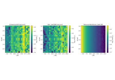
Validating the curvature engine: Einstein’s vacuum field equations
1915 – Mercury’s Perihelion Precession#
Urbain Le Verrier noticed, as early as 1859, that Mercury’s orbit precesses about 43 arcseconds per century faster than Newtonian gravity – accounting for every known planetary perturbation – could explain. The anomaly went unexplained for over half a century; a hypothetical planet, “Vulcan”, orbiting inside Mercury to account for the extra tug, was searched for and never found. On 18 November 1915, days before he finished the general theory itself, Einstein computed the correction general relativity predicts for a test mass orbiting a central body,
per orbit, where \(a\) is the orbit’s semi-major axis and \(e\) its eccentricity. Plugging in Mercury’s orbital elements reproduced the missing 43 arcseconds per century exactly. Einstein later told a colleague the result gave him heart palpitations – it was general relativity’s first successful confrontation with data, four years before Eddington’s eclipse expedition made the theory famous.
Implementation:
physicskit.relativity.chapters.schwarzschild.SchwarzschildBlackHole.weak_field_precession_per_orbit()
computes exactly this closed-form precession;
integrate_geodesic()
together with
perihelion_precession()
recovers the same number the other way, by directly integrating an
eccentric geodesic from
eccentric_orbit_initial_state()
and measuring the excess angle swept between successive perihelion
passages.
References: A. Einstein, “Erklärung der Perihelbewegung des Merkur aus der allgemeinen Relativitätstheorie,” Sitzungsberichte der Preußischen Akademie der Wissenschaften, 831-839 (18 Nov. 1915).
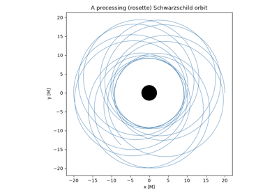
Perihelion precession: the anomaly that first confirmed General Relativity
1916 – Schwarzschild’s Exact Solution#
Weeks after Einstein’s paper appeared – and while serving as an artillery officer on the Russian front in the First World War – Karl Schwarzschild found the first exact solution to the field equations: the spacetime around a single non-rotating, spherically symmetric mass,
Schwarzschild sent his solution to Einstein, who was reportedly astonished that an exact answer existed at all. The metric’s coordinate singularity at \(r=2M\) – initially dismissed as unphysical – would only be understood decades later as an event horizon, the boundary of a black hole. Schwarzschild died of an autoimmune illness contracted at the front just a few months after publishing it.
Implementation: physicskit.relativity.core.tensors.schwarzschild_metric()
is exactly this line element;
physicskit.relativity.chapters.schwarzschild.SchwarzschildBlackHole
wraps it with the derived quantities Schwarzschild’s solution predicts –
the horizon_radius \(r_s=2M\), photon_sphere_radius
\(r_{ph}=3M\), and isco_radius \(r_{\text{ISCO}}=6M\).
References: K. Schwarzschild, “Über das Gravitationsfeld eines Massenpunktes nach der Einsteinschen Theorie,” Sitzungsberichte der Königlich Preußischen Akademie der Wissenschaften, 189-196 (1916).
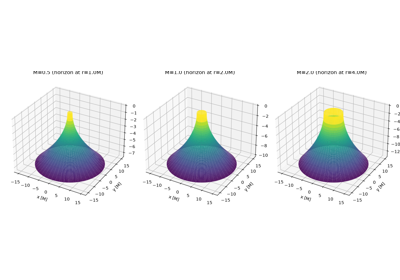
Flamm’s paraboloid: gravity as curved geometry, not a force
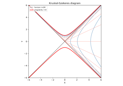
Kruskal-Szekeres and Penrose-Carter diagrams: the true shape of spacetime
1916-1918 – Einstein Predicts Gravitational Waves#
Barely a year after finishing general relativity, Einstein linearized the field equations about flat spacetime and found that they admit wave solutions: small ripples in the metric that propagate at the speed of light, sourced by a time-varying mass quadrupole moment and radiating away energy at a rate
the quadrupole formula. His first 1916 paper on the subject contained an error – a spurious factor of two from an incorrect gauge choice – which he corrected two years later in a second paper laying out the quadrupole formula essentially as it is used today. Einstein himself remained privately unsure whether the waves were physically real or merely a coordinate artifact, a question not fully settled within the relativity community until the 1950s and 1960s. It would take until 1974 for the first (indirect) astrophysical evidence that they exist, and until 2015 for a direct detection.
Implementation: physicskit.relativity.chapters.gw_merger.BinaryMerger.inspiral_frequency()
and inspiral_strain()
implement exactly this leading-order (Newtonian quadrupole) radiation
formula for a binary source, the direct numerical descendant of Einstein’s
corrected 1918 result.
References: A. Einstein, “Näherungsweise Integration der Feldgleichungen der Gravitation,” Sitzungsberichte der Königlich Preußischen Akademie der Wissenschaften, 688-696 (1916); A. Einstein, “Über Gravitationswellen,” Sitzungsberichte der Preußischen Akademie der Wissenschaften, 154-167 (1918) (correcting the 1916 paper’s factor-of-two error).
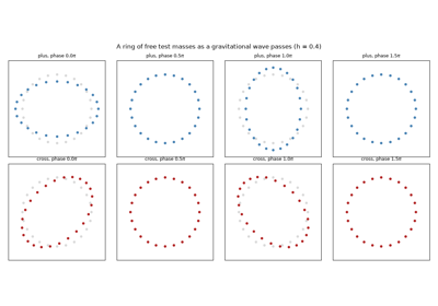
Einstein predicts gravitational waves: polarizations and the quadrupole formula
1919 – The Eddington Eclipse Expedition#
General relativity predicts that light passing near a massive body is deflected by twice the angle Newtonian gravity (treating light as a particle) would give,
for a photon with impact parameter \(b\). Frank Dyson, the Astronomer Royal, organized two expeditions to observe the total solar eclipse of 29 May 1919 – the only time stars close enough to the Sun’s limb are visible at all – so that a result from one site could be checked against the other. Arthur Eddington and Edwin Cottingham traveled to the island of Principe, while Andrew Crommelin and Charles Davidson took a second set of plates at Sobral, Brazil; contrary to the popular account that credits Eddington alone, it was Crommelin and Davidson’s Sobral data – the sharper and more numerous of the two plate sets – that gave the more decisive measurement. Both sites measured a deflection consistent with Einstein’s value, not Newton’s, and Dyson, Eddington, and Davidson jointly published the combined result. The announcement, later that year, made Einstein a household name overnight and stands as general relativity’s first observational triumph.
Implementation: physicskit.relativity.chapters.schwarzschild.SchwarzschildBlackHole.light_deflection_angle()
implements exactly this weak-field formula;
physicskit.relativity.chapters.lensing.exact_deflection_angle()
numerically integrates the full null geodesic for comparison, capturing the
strong-field corrections that become significant close to the photon
sphere, where the weak-field formula above breaks down.
References: F. W. Dyson, A. S. Eddington, and C. Davidson, “A Determination of the Deflection of Light by the Sun’s Gravitational Field, from Observations Made at the Total Eclipse of May 29, 1919,” Phil. Trans. R. Soc. A 220, 291-333 (1920) (results announced Nov. 1919; the paper itself appeared the following year).
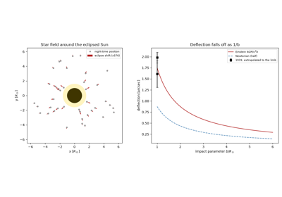
The Eddington eclipse expedition: starlight bent by the Sun
1922 – Friedmann, Lemaitre, and the Expanding Universe#
Alexander Friedmann showed, in 1922, that Einstein’s field equations admit non-static, homogeneous, isotropic cosmological solutions – in direct contradiction to Einstein’s own preference (at the time) for a static universe, which had led him to introduce the cosmological constant \(\Lambda\) specifically to prevent expansion. Georges Lemaitre independently rediscovered these solutions in 1927 and connected them to the redshifts already being observed in distant galaxies, two years before Hubble’s own 1929 observational confirmation. The Friedmann equation,
governs how the universe’s scale factor \(a(t)\) evolves under the combined gravity of radiation, matter, curvature, and dark energy.
Implementation: physicskit.relativity.core.tensors.flrw_metric()
implements the FLRW line element itself;
physicskit.relativity.chapters.cosmology.FLRWCosmology and its
hubble_parameter()
method solve exactly this Friedmann equation, with
luminosity_distance_mpc()
and age_gyr()
built on top of it.
References: A. Friedmann, “Über die Krümmung des Raumes,” Z. Phys. 10, 377-386 (1922); G. Lemaître, Annales de la Société Scientifique de Bruxelles A47, 49-59 (1927); E. Hubble, “A Relation between Distance and Radial Velocity among Extra-Galactic Nebulae,” PNAS 15(3), 168-173 (1929).
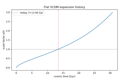
The expanding universe: Hubble’s law and the Friedmann equations
1936 – Einstein Rings and Gravitational Lensing#
Einstein had privately worked out, as early as 1912, that a massive body could act as a gravitational lens, bending and magnifying the light of a background source – but he did not publish the result until 1936, and even then considered it of little practical interest, since the angular separations involved seemed hopelessly small for any real star to resolve. When the observer, lens, and source line up exactly, the lensed image forms a complete ring around the lens, of angular radius
the Einstein radius. Any other alignment splits a single source into two images of unequal brightness. Fritz Zwicky pointed out in 1937 that entire galaxies, not just stars, could lens background sources strongly enough to observe – the first galaxy-scale lens was found in 1979, and the first complete Einstein ring imaged in 1988.
Implementation: physicskit.relativity.chapters.lensing.PointMassLens
and its einstein_angle(),
image_angles(),
and magnification()
methods solve exactly this thin-lens problem, including the Paczynski
microlensing magnification formula used in exoplanet and dark-object
surveys.
References: A. Einstein, “Lens-Like Action of a Star by the Deviation of Light in the Gravitational Field,” Science 84(2188), 506-507 (1936); F. Zwicky, “Nebulae as Gravitational Lenses,” Phys. Rev. 51, 290 (1937); first observed lens: D. Walsh, R. F. Carswell, and R. J. Weymann, Nature 279, 381-384 (1979); first Einstein ring: J. N. Hewitt et al., Nature 333, 537-540 (1988).
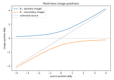
1939 – Tolman-Oppenheimer-Volkoff and Neutron Star Structure#
Richard Tolman, and then J. Robert Oppenheimer and George Volkoff, derived the relativistic generalization of Newtonian hydrostatic equilibrium for a self-gravitating fluid sphere – the equation describing the interior structure of a neutron star, matter compressed to nuclear density and held up against collapse purely by neutron degeneracy pressure. Unlike the Newtonian case, the TOV equation predicts a maximum possible mass: past a critical central density, adding more matter only accelerates collapse, and no degeneracy pressure can halt it – the star must become a black hole. This maximum mass (loosely, the “Tolman-Oppenheimer-Volkoff limit”) remains an active area of nuclear-equation-of-state research today.
Implementation: physicskit.relativity.chapters.neutron_star.NeutronStar
and its solve()
method integrate exactly the TOV equations outward from the stellar center
to the surface;
mass_radius_curve()
traces out the resulting mass-radius relation and its maximum-mass turning
point.
References: R. C. Tolman, “Static Solutions of Einstein’s Field Equations for Spheres of Fluid,” Phys. Rev. 55, 364-373 (1939); J. R. Oppenheimer and G. M. Volkoff, “On Massive Neutron Cores,” Phys. Rev. 55, 374-381 (1939).
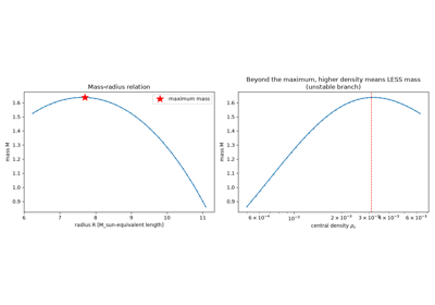
The neutron star maximum mass: solving the TOV equations
1963 – Kerr’s Rotating Black Hole Solution#
For nearly fifty years after Schwarzschild, no one found an exact solution describing a rotating black hole – the astrophysically realistic case, since essentially every collapsing star has some angular momentum. Roy Kerr found one in 1963, characterized by just two parameters, mass \(M\) and spin \(a=J/M\). The Kerr solution predicts frame dragging: spacetime itself is dragged around the rotating hole, so strongly near the horizon that no observer, however powerful their engine, can remain at fixed angular position within the ergosphere – the region \(r_+ < r < M+\sqrt{M^2-a^2\cos^2\theta}\) outside the horizon where this effect appears.
Implementation: physicskit.relativity.core.tensors.kerr_metric_bl()
implements the Kerr metric in Boyer-Lindquist coordinates;
physicskit.relativity.chapters.kerr.KerrBlackHole and its
frame_dragging_angular_velocity()
and ergosphere_radius()
methods compute exactly these effects, and
isco_radius()
gives the spin-dependent innermost stable circular orbit.
References: R. P. Kerr, “Gravitational Field of a Spinning Mass as an Example of Algebraically Special Metrics,” Phys. Rev. Lett. 11, 237-238 (1963).
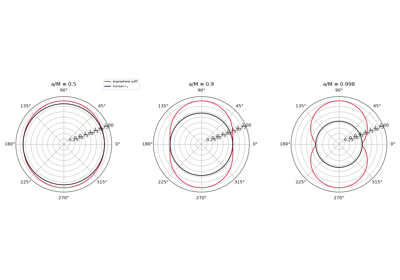
Frame dragging and the ergosphere of a Kerr black hole
1965 – The Kerr-Newman Black Hole and Carter’s Fourth Constant#
Two years after Kerr’s rotating solution, Ezra Newman and five co-authors applied a complex coordinate transformation to the Reissner-Nordström metric and obtained a rotating black hole that also carries electric charge. In Boyer-Lindquist coordinates it is the Kerr metric with
so Schwarzschild, Reissner-Nordström and Kerr are its special cases, and the no-hair theorems of the following decade showed that it is the most general stationary black hole of Einstein-Maxwell theory: mass, spin and charge are all an outside observer can measure. Brandon Carter (1968) found that the Hamilton-Jacobi equation of a charged test particle still separates. This gives a fourth constant of motion beyond energy, angular momentum and mass, and the radial and polar motions decouple,
Photons on spherical orbits, \(R = R' = 0\), outline the shadow; charge, like spin, shrinks it, and its shape constrains the charge of the black holes imaged by the Event Horizon Telescope.
Implementation: physicskit.relativity.chapters.kerr_newman.KerrNewmanBlackHole
gives the horizons, the spherical and equatorial photon orbits and the
analytic shadow edge;
geodesic()
integrates Carter’s equations for photons and charged massive particles,
and
ray_traced_shadow()
ray-traces the shadow to check the edge.
References: E. T. Newman, E. Couch, K. Chinnapared, A. Exton, A. Prakash and R. Torrence, J. Math. Phys. 6, 918-919 (1965); B. Carter, Phys. Rev. 174, 1559-1571 (1968); J. M. Bardeen, in Black Holes (Les Houches 1972), 215-239 (1973); A. de Vries, Class. Quantum Grav. 17, 123-144 (2000).

The Kerr-Newman black hole: geodesics and the shadow of a charged, rotating hole
1965 – Penrose’s Singularity Theorems#
Schwarzschild’s \(r=0\) singularity and the FLRW big bang had both appeared inside solutions with an enormous amount of built-in symmetry, leading many, including Einstein himself, to suspect that singularities were merely an artifact of that idealized symmetry – an assumption that real, lumpy, rotating collapsing matter would surely avoid. Roger Penrose proved otherwise in 1965: using global, topological methods rather than solving the field equations explicitly, he showed that once a trapped surface forms – a closed surface from which even outgoing light rays are converging inward – and ordinary energy conditions hold, at least one causal geodesic in the resulting spacetime must be incomplete. No symmetry assumption is needed. For a simple, spherically symmetric illustration of that incompleteness, a particle dropped from rest at radius \(R\) reaches the singularity in finite proper time,
rather than taking forever, as a merely coordinate-induced artifact would. Stephen Hawking adapted the same methods to the time-reversed case the following year, showing an initial big-bang singularity is likewise unavoidable given only that the universe contains enough matter and is expanding. Penrose received a share of the 2020 Nobel Prize in Physics “for the discovery that black hole formation is a robust prediction of the general theory of relativity.”
Implementation:
physicskit.relativity.chapters.schwarzschild.SchwarzschildBlackHole.eccentric_orbit_initial_state()
with eccentricity_boost=1.0 starts a geodesic at rest – zero angular
velocity – at radius \(r_0\);
integrate_geodesic()
evolves it inward and shows the elementary, coordinate-bound version of
the puzzle directly: the particle’s own proper time \(\tau\) climbs
smoothly and stays finite all the way to the horizon, while
\(dt/d\tau\) grows without bound over the same interval – Schwarzschild
coordinates are singular exactly at \(r=2M\), so this coordinate-time
integrator cannot be pushed past the horizon at all. Reaching the true
singularity needs the closed-form \(\tau_{r=0}\) above, evaluated
directly from the same radial energy-conservation equation the integrator
solves, independent of which time coordinate is used to parametrize the
fall – not a further numerical integration past the point where these
particular coordinates break down.
References: R. Penrose, “Gravitational Collapse and Space-Time Singularities,” Phys. Rev. Lett. 14, 57-59 (1965); S. W. Hawking, “Singularities in the Universe,” Proc. R. Soc. A 294, 511-521 (1966).
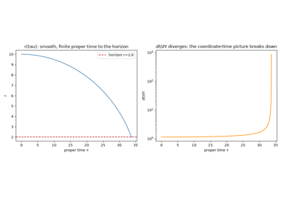
Penrose’s singularity theorems: finite proper time, divergent coordinate time
1969 – Penrose’s Energy-Extraction Process#
Roger Penrose showed that the ergosphere is not just a curiosity of rotating spacetime but a genuine energy resource: inside it, the timelike Killing vector associated with time-translation symmetry becomes spacelike, so a particle there can have negative energy as measured by an observer at infinity. If a particle entering the ergosphere splits in two, with one negative-energy fragment falling into the horizon, energy conservation forces the escaping fragment to carry away more energy than the original particle had – extracting rotational energy from the black hole itself. The process is capped by Hawking’s area theorem: the hole’s irreducible mass, \(M_{\text{irr}}=\sqrt{Mr_+/2}\), can never decrease, limiting the maximum extractable fraction to about 29% for a maximally spinning hole.
Implementation: physicskit.relativity.chapters.kerr.KerrBlackHole.penrose_energy_gain()
computes the escaping fragment’s energy gain for a given ergosphere split;
max_penrose_efficiency()
gives exactly this 29%-at-extremal-spin efficiency ceiling.
References: R. Penrose, “Gravitational Collapse: The Role of General Relativity,” Rivista del Nuovo Cimento, Numero Speciale I, 252-276 (1969).
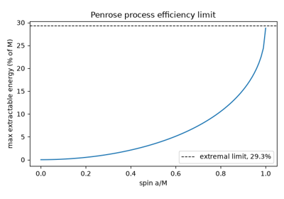
The Penrose process: extracting a black hole’s rotational energy
1959-1962 – The ADM (3+1) Formalism#
Chronologically, the ADM formalism predates the Kerr and Penrose results above; it is placed here instead because it belongs thematically with the numerical-relativity thread this chronology picks back up at 1974 and, decisively, in 2005. Richard Arnowitt, Stanley Deser, and Charles Misner recast general relativity as an initial-value problem: instead of treating spacetime as a single four-dimensional block satisfying the field equations everywhere at once, they sliced it into a stack of spacelike three-dimensional hypersurfaces, each carrying a spatial metric \(\gamma_{ij}\) and extrinsic curvature \(K_{ij}\), related to their neighbors by a lapse function \(\alpha\) and shift vector \(\beta^i\) that describe how the slicing threads through spacetime. Einstein’s ten field equations split into evolution equations for \(\gamma_{ij}\) and \(K_{ij}\) plus four constraint equations (Hamiltonian and momentum) that must hold on every slice. This “3+1” decomposition – three spatial dimensions evolving in a time coordinate – is the starting point of essentially every numerical-relativity simulation since, including the codes that produced the 2005 binary-black-hole-merger breakthrough below and, decades later, the waveform templates behind LIGO’s detections.
Connection: physicskit.relativity does not itself implement a 3+1
evolution scheme – every metric here (Schwarzschild, Kerr, FLRW) is
treated as a known analytic background rather than evolved numerically
from initial data, so there is no lapse/shift/extrinsic-curvature
machinery to point to. The package’s role in this chronology begins one
step downstream of ADM, with the merger outcomes – remnant mass, spin,
and ringdown – that full numerical-relativity evolutions of the ADM
equations first computed; see the 2005 entry below and
physicskit.relativity.chapters.gw_merger.BinaryMerger.
References: R. Arnowitt, S. Deser, and C. W. Misner, “The Dynamics of General Relativity,” in Gravitation: An Introduction to Current Research, ed. L. Witten (Wiley, 1962), pp. 227-265; originally developed in a series of Physical Review papers, e.g. R. Arnowitt, S. Deser, and C. W. Misner, “Dynamical Structure and Definition of Energy in General Relativity,” Phys. Rev. 116, 1322 (1959).
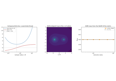
The ADM (3+1) formalism: black-hole initial data and the ADM mass
1974 – The Hulse-Taylor Binary Pulsar#
General relativity predicts that any accelerating mass quadrupole radiates gravitational waves, carrying away orbital energy – but the effect is so weak that no laboratory source could ever hope to detect it directly. Russell Hulse and Joseph Taylor found an astrophysical source strong enough to reveal the effect indirectly: PSR B1913+16, a pulsar in a tight orbit with another neutron star, discovered in 1974. Over the following years, precise pulsar timing showed the pair’s orbital period shrinking at exactly the rate
predicted by Peters’ 1964 formula for gravitational-wave energy loss. The pulsar was discovered in 1974; Taylor and Weisberg’s landmark timing analysis, published in 1982, already showed the orbital decay tracking general relativity’s prediction to about 1%, and later refinements of the same pulsar-timing dataset – Taylor and Weisberg again in 1989, and Weisberg and Taylor’s subsequent updates through the mid-2000s – tightened the agreement to the oft-quoted 0.2% figure. Together this stood as the first evidence, albeit indirect, that gravitational waves are real. Hulse and Taylor received the 1993 Nobel Prize in Physics for the discovery.
Implementation: physicskit.relativity.chapters.gw_merger.BinaryMerger.semi_major_axis_decay_rate()
implements exactly this Peters-formula orbital shrinkage rate;
period_decay_rate()
converts it to the observable \(dP/dt\) that Hulse and Taylor measured.
References: R. A. Hulse and J. H. Taylor, “Discovery of a Pulsar in a Binary System,” ApJ Letters 195, L51-L53 (1975) (discovered 1974, published 1975); P. C. Peters, “Gravitational Radiation and the Motion of Two Point Masses,” Phys. Rev. 136, B1224-B1232 (1964); J. H. Taylor and J. M. Weisberg, “A New Test of General Relativity: Gravitational Radiation and the Binary Pulsar PSR 1913+16,” ApJ 253, 908-920 (1982) (~1% agreement); J. H. Taylor and J. M. Weisberg, “Further Experimental Tests of Relativistic Gravity Using the Binary Pulsar PSR 1913+16,” ApJ 345, 434-450 (1989) and subsequent Weisberg & Taylor updates (~2004-2010) for the tighter ~0.2% figure.
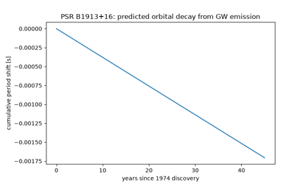
The Hulse-Taylor binary pulsar: the first (indirect) evidence for gravitational waves
1976 – Gravity Probe A and Relativistic Timekeeping#
General relativity predicts that a clock deeper in a gravitational potential runs slower than one farther out – gravitational time dilation. Robert Vessot and Martin Levine put this to its most precise test yet in June 1976, launching a hydrogen maser clock on a suborbital rocket to 10,000 km altitude and comparing its rate against an identical clock on the ground throughout the flight: the Gravity Probe A experiment confirmed the predicted rate shift to about one part in 10,000. The rocket flew in June 1976, but the definitive analysis was not published until four years later – Vessot, Levine, and collaborators’ 1980 paper is the citation behind the “1976” result, and readers looking for a contemporaneous 1976 paper will not find one. That same effect is not merely a laboratory curiosity today – every GPS satellite clock runs measurably faster than clocks on the ground it serves, and the discrepancy must be corrected for by design, or accumulated position errors would reach several kilometers per day.
Implementation: physicskit.relativity.chapters.timekeeping.clock_rate_factor()
computes exactly this relativistic clock-rate shift for an orbiting clock;
gps_relativistic_offset_per_day()
gives the resulting daily timing correction GPS satellites apply.
References: R. F. C. Vessot, M. W. Levine, et al., “Test of Relativistic Gravitation with a Space-Borne Hydrogen Maser,” Phys. Rev. Lett. 45, 2081-2084 (1980) (experiment flown June 1976, results published 1980).
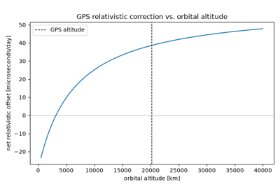
2005-2006 – Numerical Relativity Solves the Binary Black Hole Merger#
For thirty years after the ADM formalism made numerical evolution of the field equations possible in principle, every attempt to simulate two black holes spiraling together and merging crashed before reaching merger – numerical instabilities, chiefly around the singularities themselves, grew without bound and destroyed the simulation. Frank Pretorius broke the deadlock in 2005 with a new formulation (generalized harmonic coordinates, combined with excision of the singular region) that evolved a binary black hole cleanly through inspiral, merger, and ringdown for the first time. Within months, two independent groups – Campanelli, Lousto, Marronetti, and Zlochower, and separately Baker, Centrella, Choi, Koppitz, and van Meter – found a second, more broadly adopted route to the same result, the “moving puncture” method, which let punctures representing the black holes move freely across the numerical grid without the manual excision Pretorius’s approach required. Together these breakthroughs turned binary black hole mergers from an analytically inaccessible strong-field problem into a solvable one, making it possible, for the first time, to compute the full inspiral-merger-ringdown waveform – including the merger itself, which no post-Newtonian or perturbative approximation can reach – directly from the field equations. The precomputed template banks and surrogate waveform models this made possible are exactly what let LIGO recognize GW150914 as a binary black hole merger the moment it arrived, a decade later.
Implementation: physicskit.relativity.chapters.gw_merger.BinaryMerger.remnant_estimate()
anchors its equal-mass, non-spinning endpoint (\(M_f \approx 0.95 M\),
\(a_f/M_f \approx 0.69\)) to exactly the merger remnant mass and spin
that these numerical-relativity simulations first measured; this package’s
own docstring is explicit that remnant_estimate() is “not a
precision numerical-relativity surrogate” but a simple interpolation
toward that well-measured NR result, and
full_waveform()
stitches an inspiral onto a quasinormal-mode ringdown into the same
qualitative inspiral-merger-ringdown structure that these simulations were
the first to compute in full.
References: F. Pretorius, “Evolution of Binary Black-Hole Spacetimes,” Phys. Rev. Lett. 95, 121101 (2005); M. Campanelli, C. O. Lousto, P. Marronetti, and Y. Zlochower, “Accurate Evolutions of Orbiting Black-Hole Binaries without Excision,” Phys. Rev. Lett. 96, 111101 (2006); J. G. Baker, J. Centrella, D.-I. Choi, M. Koppitz, and J. van Meter, “Gravitational-Wave Extraction from an Inspiraling Configuration of Merging Black Holes,” Phys. Rev. Lett. 96, 111102 (2006).
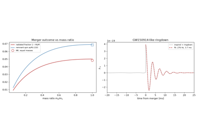
Numerical relativity solves the binary black hole merger
2015 – LIGO and the Direct Detection of Gravitational Waves#
On 14 September 2015, the twin LIGO detectors observed a transient signal – a rising “chirp” in frequency and amplitude followed by a brief ringdown – matching, to remarkable precision, the predicted waveform of two black holes of roughly 36 and 29 solar masses spiraling together and merging into a single, still-quivering black hole, radiating about three solar masses’ worth of energy as gravitational waves in a fraction of a second. GW150914 was the first direct detection of gravitational waves, a full century after Einstein predicted their existence, and the first direct observation of a binary black hole merger. The 2017 Nobel Prize in Physics recognized the LIGO detection.
Implementation: physicskit.relativity.chapters.gw_merger.BinaryMerger
implements exactly this inspiral-merger-ringdown sequence:
inspiral_strain()
gives the chirping inspiral waveform,
qnm_frequency_damping()
and ringdown_strain()
give the remnant’s damped-sinusoid ringdown, and
full_waveform()
stitches the two regimes together into a single GW150914-like signal.
References: B. P. Abbott et al. (LIGO Scientific Collaboration and Virgo Collaboration), “Observation of Gravitational Waves from a Binary Black Hole Merger,” Phys. Rev. Lett. 116, 061102 (2016).
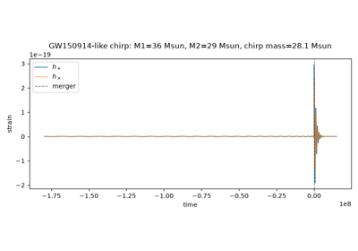
GW150914: the first direct detection of gravitational waves
2017 – GW170817 and the Dawn of Multi-Messenger Astronomy#
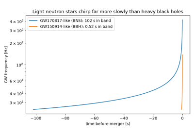
On 17 August 2017, LIGO and Virgo detected the inspiral of a binary neutron star system – far lighter than any binary black hole seen before, and correspondingly slower-chirping, remaining in the detectors’ sensitive band for over a minute rather than a fraction of a second. Just 1.7 seconds after the merger, the Fermi and INTEGRAL satellites detected a short gamma-ray burst from the same patch of sky, and observatories worldwide went on to track the fading kilonova afterglow for weeks – confirming that short gamma-ray bursts are neutron-star mergers, and that these mergers forge heavy elements like gold and platinum via rapid neutron capture (the r-process), long suspected but never before directly observed. It was the first gravitational-wave event with a confirmed electromagnetic counterpart, opening the era of multi-messenger astronomy, and its independently measured distance and inferred recession velocity gave a new, “standard siren” measurement of the Hubble constant. The measured chirp mass,
was immediately recognizable as two neutron stars rather than two black holes: far below any black hole binary LIGO had detected, and consistent with the narrow mass range neutron stars are observed to occupy.
Implementation: physicskit.relativity.chapters.gw_merger.BinaryMerger
with \(m_1, m_2 \approx 1.4\,M_\odot\) reproduces this chirp mass via
its chirp_mass
property, and its inspiral_frequency()
sweep shows exactly why such light neutron stars chirp for so much longer
than GW150914’s ~30-solar-mass black holes did – long enough for the
joint gravitational-wave and gamma-ray sky localization that made the
electromagnetic follow-up possible; the mass-radius relation from
physicskit.relativity.chapters.neutron_star.NeutronStar traced by
mass_radius_curve()
is exactly the equation-of-state relation that observations like
GW170817’s tidal deformability measurement are used to constrain.
References: B. P. Abbott et al. (LIGO Scientific Collaboration and Virgo Collaboration), “GW170817: Observation of Gravitational Waves from a Binary Neutron Star Inspiral,” Phys. Rev. Lett. 119, 161101 (2017); multi-messenger follow-up: “Multi-messenger Observations of a Binary Neutron Star Merger,” ApJ Letters 848, L12 (2017).
2019 – Event Horizon Telescope: The First Black Hole Image#
On 10 April 2019, the Event Horizon Telescope collaboration released the first direct image of a black hole’s shadow: the supermassive black hole at the center of the galaxy M87, roughly 6.5 billion solar masses, imaged by linking radio dishes across the globe into a single Earth-diameter interferometer. The image showed a dark central shadow ringed by bright, asymmetric emission from infalling plasma – direct visual confirmation of the photon sphere and the shadow it casts, exactly as general relativity predicts, cast at a distance \(D\) at angular radius
The collaboration went on to image Sagittarius A*, the far smaller and closer supermassive black hole at the center of our own galaxy, in 2022. Reinhard Genzel and Andrea Ghez shared the other half of the 2020 Nobel Prize in Physics for tracking stellar orbits around Sagittarius A* closely enough, over decades, to establish that it must be an extremely compact, extremely massive dark object.
Implementation:
physicskit.relativity.chapters.schwarzschild.SchwarzschildBlackHole.critical_impact_parameter
gives exactly this shadow-casting impact parameter \(b_c=3\sqrt3\,M\);
physicskit.relativity.core.raytracer.render_shadow_image() and its
rotating-black-hole counterpart
render_kerr_shadow_image()
backward ray-trace this shadow-and-photon-ring signature pixel by pixel
from a virtual camera, and
plot_black_hole_shadow()
renders the result, reproducing the qualitative dark-disk-with-bright-ring
appearance of the EHT’s M87* and Sagittarius A* images.
References: Event Horizon Telescope Collaboration, “First M87 Event Horizon Telescope Results. I. The Shadow of the Supermassive Black Hole,” ApJ Letters 875, L1 (2019) (first of a six-paper series); Sgr A* results: Event Horizon Telescope Collaboration, “First Sagittarius A* Event Horizon Telescope Results. I. The Shadow of the Supermassive Black Hole in the Center of the Milky Way,” ApJ Letters 930, L12 (2022).
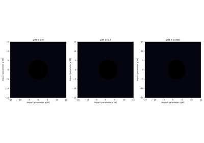
The Kerr shadow: a rotating black hole’s asymmetric silhouette
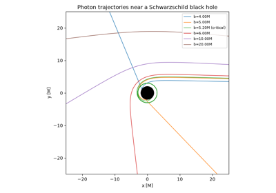
The black hole shadow: from the photon sphere to the Event Horizon Telescope