Breakthroughs in Quantum Mechanics#
“I think I can safely say that nobody understands quantum mechanics.” – Richard Feynman, The Character of Physical Law, 1965
Quantum mechanics replaced a world of definite trajectories with one of
wavefunctions, probabilities, and operators – and did so not as a single
discovery but as a three-decade argument among the physicists who built it,
from Planck’s reluctant quantum in 1900 to Bell’s 1964 proof that no
“common-sense” theory could ever reproduce its predictions. The chronology
behind physicskit.quantum follows that argument in order: the old
quantum theory of Bohr, the two rival (and ultimately equivalent)
mechanics of Heisenberg and Schrodinger, the interpretive battles over
what the wavefunction even means, and the exactly solvable model
problems – the hydrogen atom, the harmonic oscillator, the square well –
that remain the field’s working vocabulary today. This chronology traces
that thread, with a pointer to the corresponding implementation in this
package at each stop.
1900 – Planck’s Quantum Hypothesis#
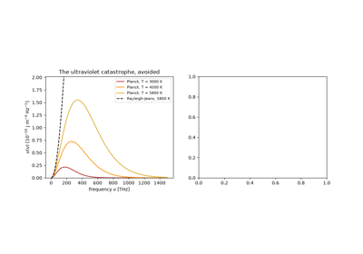
To fit the observed spectrum of blackbody radiation – which classical electrodynamics predicted should diverge at short wavelengths (the “ultraviolet catastrophe”) – Max Planck proposed, in a December 1900 paper to the German Physical Society, that the energy exchanged between radiation and matter is not continuous but comes in discrete quanta,
for an oscillator of frequency \(\nu\). Planck himself considered this a mathematical device rather than a physical claim – he later called it “an act of desperation” – but the idea that a harmonic oscillator’s energy spectrum is discrete, evenly spaced by \(h\nu\) (or, in the full quantum treatment developed a generation later, by \(\hbar\omega\)), turned out to be exactly right, and became the seed of everything that follows in this chronology.
Connection: physicskit.quantum.chapters.harmonic_spin.HarmonicOscillator.energy()
returns exactly this evenly spaced spectrum, \(E_n = \hbar\omega(n +
\tfrac12)\), for the quantum harmonic oscillator that eventually made
Planck’s quantization rule precise.
References: M. Planck, Verhandlungen der Deutschen Physikalischen Gesellschaft 2, 237-245 (1900).
Planck’s quantum hypothesis and blackbody radiation
1913 – Bohr’s Atomic Model#
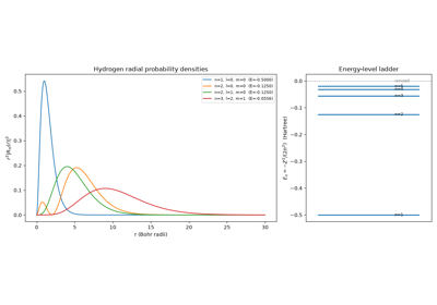
Niels Bohr proposed that an electron orbiting a nucleus is restricted to a discrete set of “stationary states” with quantized angular momentum \(L = n\hbar\), in which – contrary to classical electrodynamics – it does not radiate, jumping between orbits only by emitting or absorbing a photon of energy \(\Delta E\). For hydrogen this postulate, combined with a classical circular-orbit force balance, gives the energy levels
reproducing the empirical Rydberg formula for hydrogen’s spectral lines to remarkable precision. Bohr’s model was frankly ad hoc – a classical orbit with a quantization rule bolted on – but it was the first successful quantum theory of an atom, and every one of its energy levels survives unchanged in the exact 1926 treatment that replaced it.
Connection: physicskit.quantum.chapters.hydrogen_am.HydrogenOrbital
reproduces Bohr’s \(n\)-dependence exactly in its energy property,
\(E_n = -Z^2/(2n^2)\), even though it is derived from the full
Schrodinger equation rather than Bohr’s semiclassical orbits. See it in
Hydrogen orbitals.
References: N. Bohr, “On the Constitution of Atoms and Molecules,” Phil. Mag. Ser. 6, 26, 1-25, 476-502, 857-875 (1913).
1913 – The Zeeman and Stark Effects#
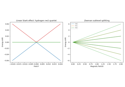
Pieter Zeeman had already shown, in 1896, that spectral lines split into several components in a magnetic field (Nobel Prize, 1902, shared with Hendrik Lorentz, who supplied the classical explanation). In 1913 Johannes Stark discovered the electrical analogue: hydrogen’s Balmer lines split linearly under a strong external electric field. Both effects became essential tools of “old quantum theory” spectroscopy, and both later became textbook applications of perturbation theory – the Zeeman effect of non-degenerate perturbation theory, and the linear Stark effect of hydrogen specifically of the degenerate variety, made possible only by hydrogen’s accidental level degeneracy in \(l\).
Implementation: physicskit.quantum.chapters.perturbation.zeeman_splitting()
and zeeman_spectrum()
compute the first-order Zeeman sublevel shifts;
linear_stark_shift() and
stark_n2_quartet()
reproduce the classic linear Stark quartet of hydrogen’s \(n=2\) shell.
References: P. Zeeman, Phil. Mag. 43, 226-239 (1897) (originally published in Dutch in 1896); J. Stark, Sitzungsber. Preuss. Akad. Wiss. 1913, 932-946.
Stark and Zeeman splitting: static perturbation theory
1915-1916 – Wilson-Sommerfeld Quantization#
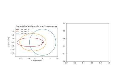
William Wilson and Arnold Sommerfeld independently generalized Bohr’s quantization rule from circular orbits to any periodic classical motion, replacing it with the phase-space integral
taken once around a full period. Applied to elliptical Kepler orbits this reproduced hydrogen’s Bohr energies unchanged (adding a second quantum number for orbital shape), and Sommerfeld’s relativistic refinement of the same rule correctly predicted hydrogen’s fine structure – an early triumph of “old quantum theory.” But the rule only quantizes systems whose classical motion is periodic and separable; it could not be extended to the helium atom or to molecular spectra, a failure that motivated the wholesale replacement Heisenberg and Schrodinger supplied over a decade later.
Connection: physicskit.semiclassical.core.wkb.bohr_sommerfeld_energies()
implements the modern, Maslov-corrected descendant of this same
phase-space quantization integral,
\(\int_{x_1}^{x_2}p\,dx=(n+\tfrac12)\pi\hbar\), turning Wilson and
Sommerfeld’s postulate into a working numerical bound-state solver for an
arbitrary one-dimensional potential.
References: W. Wilson, Phil. Mag. 29, 795-802 (1915); A. Sommerfeld, Ann. Phys. 356(17), 1-94 (1916).
Wilson-Sommerfeld quantization: elliptical orbits and fine structure
1922 – The Stern-Gerlach Experiment#
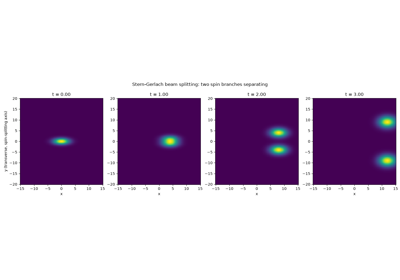
Otto Stern proposed, and with Walther Gerlach carried out at the University of Frankfurt, an experiment to test whether the “space quantization” of old quantum theory – the claim that an atom’s magnetic moment can point only along a discrete set of directions relative to an external field, rather than any classical angle – was physically real rather than a mathematical bookkeeping device. They sent a beam of silver atoms, each with one unpaired valence electron, through a strongly inhomogeneous magnetic field: a magnetic moment free to point at any angle should smear the beam into one broadened band, while a moment restricted to a discrete set of orientations should split it into a corresponding number of separate spots. In the early hours of 8 February 1922 they found the beam split cleanly in two – not smeared, confirming that spatial quantization is real, though the number of spots (two, not the odd count old quantum theory’s integer orbital angular momentum would have implied for silver’s ground state) could only be explained after Uhlenbeck and Goudsmit posited electron spin three years later, in 1925.
the spin-dependent transverse force – its sign set by which way the atom’s magnetic moment projects along the field gradient – that pushes the two spin branches apart into separately resolved lobes. Stern received the 1943 Nobel Prize in Physics for the molecular-beam method this experiment inaugurated; Gerlach, who did much of the hands-on experimental work (including the slit refinement that made the clean February 1922 result possible), was never awarded a share, a historical omission usually attributed to wartime politics rather than to any dispute over credit.
Implementation: physicskit.quantum.chapters.spin.SternGerlach
implements the standard semiclassical two-branch treatment: each spin
projection is modeled as an independent Gaussian wavepacket subject to
exactly this constant transverse force, so its
joint_density() (and
its time-stacked
joint_density_stack())
show the two lobes separating in real time as the beam propagates through
the apparatus, animated with
animate_density_2d().
See it in The Stern-Gerlach experiment.
References: W. Gerlach and O. Stern, Z. Phys. 9, 349-352 (1922); precursor O. Stern, Z. Phys. 7, 249-253 (1921).
1924 – de Broglie’s Matter Waves#
In his doctoral thesis, Louis de Broglie proposed that the wave-particle duality Einstein had already established for light should run in reverse: every material particle of momentum \(p\) has an associated wavelength
The hypothesis was speculative – de Broglie had no direct evidence for it – until Davisson and Germer observed electron diffraction from a nickel crystal in 1927, confirming it experimentally. De Broglie’s wave is the first appearance of the traveling-wave factor \(e^{ikx}\) that appears in every wavepacket and plane-wave state used throughout quantum mechanics.
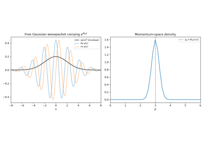
Implementation: physicskit.quantum.chapters.wave_packets.free_gaussian_wavepacket()
builds a localized wavepacket carrying exactly this de Broglie phase,
\(e^{ik_0 x}\), modulating a Gaussian envelope centered on momentum
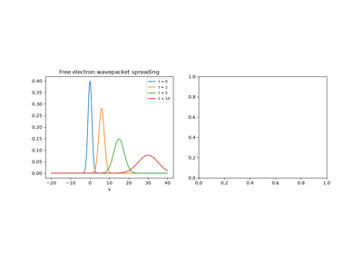
\(p_0 = \hbar k_0\). The same packet’s subsequent free evolution –
GaussianDispersion, the
exact analytic solution of the free-particle Schrodinger equation for a
Gaussian initial condition – is animated frame by frame with its
trajectory()
method and animate_density(),
showing the de Broglie phase riding along a center that advances
ballistically at \(v=\hbar k_0/m\) while the envelope spreads. The
animated dispersion is shown in
Jönsson’s electron double slit: interference one electron at a time.
WignerVisualizer
renders the same packet’s Wigner phase-space distribution directly, a
single blob centered on \((x_0, p_0)\) that is position space and
momentum space at once – the modern phase-space picture of exactly the
wave-particle duality de Broglie proposed.
References: L. de Broglie, Ann. Phys. (Paris) 10e série, 3 (1925) (thesis defended 1924); experimental confirmation C. Davisson and L. Germer, Phys. Rev. 30, 705-740 (1927).
1925-1927 – Pauli’s Exclusion Principle and Spin Matrices#
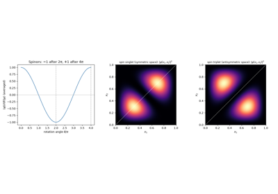
Wolfgang Pauli proposed, in 1925, that no two electrons in an atom can share the same complete set of quantum numbers – the exclusion principle that finally explained the shell structure of the periodic table old quantum theory could only fit by hand. Two years later he made the electron’s spin degree of freedom, already inferred by Uhlenbeck and Goudsmit from the Stern-Gerlach result, mathematically explicit, representing a spin-1/2 particle’s two-valued internal state with a set of three \(2\times2\) matrices,
satisfying \(\sigma_i\sigma_j = \delta_{ij}I + i\epsilon_{ijk}\sigma_k\). The exclusion principle is a statement about many-electron wavefunctions (their required antisymmetry under particle exchange, a connection Pauli himself only made fully explicit with the 1940 spin-statistics theorem); the Pauli matrices, by contrast, are the working algebra of any single two-level quantum system, and appear throughout this package wherever a spin-1/2 or qubit degree of freedom is modeled.
Implementation: physicskit.quantum.core.operators.sigma_x,
sigma_y, and
sigma_z are exactly these three
matrices, and spin_operator()
generalizes them to arbitrary spin quantum number \(s\). They are the
computational basis for two-level physics elsewhere in this chronology:
physicskit.quantum.chapters.spin.RabiProblem builds its RWA
Hamiltonian and propagator directly from sigma_z and sigma_x, and
physicskit.quantum.chapters.entanglement.BellCorrelations uses the
same two matrices to build its spin-projection measurement operators. The
exclusion principle itself – multi-electron antisymmetrization – has no
direct counterpart in this package, which works throughout in the
single- and two-qubit/single-particle regime.
References: W. Pauli, “Uber den Zusammenhang des Abschlusses der Elektronengruppen im Atom mit der Komplexstruktur der Spektren,” Z. Phys. 31, 765-783 (1925) (exclusion principle); W. Pauli, “Zur Quantenmechanik des magnetischen Elektrons,” Z. Phys. 43, 601-623 (1927) (spin matrices).
1926 – Schrodinger’s Wave Equation and the Hydrogen Atom#
Erwin Schrodinger, seeking a wave equation whose stationary states would reproduce Bohr’s energy levels, published the time-independent equation
in a rapid sequence of four papers in 1926, and immediately solved it exactly for the Coulomb potential – recovering Bohr’s hydrogen spectrum \(E_n = -Z^2/(2n^2)\) not as a postulate but as an eigenvalue, together with the full three-dimensional orbital structure Bohr’s model could never supply. Within months Schrodinger also showed his wave mechanics to be mathematically equivalent to Heisenberg’s matrix mechanics, unifying the two independently-discovered quantum theories.
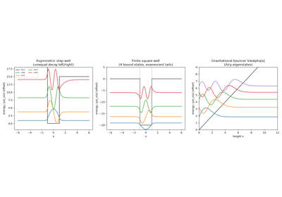
Implementation: physicskit.quantum.core.eigensolvers.NumerovSolver
solves exactly this time-independent equation numerically for an arbitrary
1D potential; physicskit.quantum.chapters.hydrogen_am.radial_wavefunction()
and spherical_harmonic()
give the exact analytic 3D hydrogen solution
\(\psi_{nlm}=R_{nl}(r)Y_l^m(\theta,\phi)\). A coherent superposition of
two such eigenstates is no longer stationary:
orbital_superposition_psi()
and orbital_superposition_density()
evolve \(\psi = c_a\psi_a e^{-iE_a t/\hbar}+c_b\psi_b e^{-iE_b t/\hbar}\)
and show its density beating at the Bohr transition frequency
\(\omega_{ab}=(E_a-E_b)/\hbar\), rendered as a Plotly play-button
isosurface animation by
animate_orbital_beating(). The
exact hydrogen solution, including the beating animation, is shown in
Hydrogen orbitals.
References: four “Mitteilungen” papers, E. Schrodinger, Ann. Phys. 384(4), 361-376; 384(6), 489-527; 385(13), 437-490; 386(18), 109-139 (1926); equivalence proof, Ann. Phys. 384(8), 734-756 (1926).
1926 – Born’s Probabilistic Interpretation#
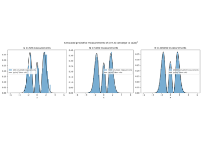
While working out scattering theory, Max Born proposed that Schrodinger’s wavefunction \(\psi\) has no direct physical reality itself; rather, \(\lvert\psi(x)\rvert^2\) is a probability density for finding the particle at \(x\) upon measurement,
This “Born rule” was the interpretive break that made quantum mechanics irreducibly statistical – not merely as a matter of incomplete knowledge, as in classical statistical mechanics, but as a fundamental feature of nature – a conclusion Einstein famously never accepted (“God does not play dice”). Born received the Nobel Prize for this insight in 1954.
Implementation: physicskit.quantum.utils.measure.simulate_position_measurement()
draws simulated measurement outcomes directly from the Born rule,
\(x_i \sim \lvert\psi(x)\rvert^2\);
position_expectation() computes the
resulting expectation value \(\langle x\rangle\).
References: M. Born, Z. Phys. 37, 863-867 (1926), corrected and extended in Z. Phys. 38, 803-827 (1926).
1926 – Born’s Collision Theory and the Born Approximation#
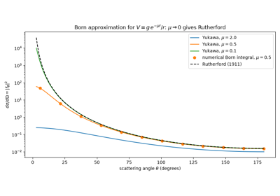
The same 1926 papers that introduced the probability interpretation (the entry above) were about collisions, and they introduced the method still used to calculate them. Born solved the scattering problem iteratively, treating the potential as a perturbation of the free incoming wave. To first order the scattering amplitude is the Fourier transform of the potential at the momentum transfer \(\mathbf q = \mathbf k' - \mathbf k\),
For a Coulomb potential it gives exactly Rutherford’s 1911 cross section, \(d\sigma/d\Omega = (Z_1Z_2e^2/4E)^2/\sin^4(\theta/2)\), a coincidence of the \(1/r\) potential that explained why Rutherford’s classical calculation had worked. The Born series is the ancestor of the perturbative expansions of quantum field theory, where the first Born approximation is a single Feynman diagram.
Implementation: physicskit.quantum.chapters.scattering.born_amplitude()
evaluates the Born integral numerically for any central potential;
yukawa_born_amplitude() is
the closed form for the screened Coulomb potential, whose unscreened limit
reproduces physicskit.particle.scattering.rutherford_dsigma_domega().
References: M. Born, “Quantenmechanik der Stossvorgange,” Z. Phys. 38, 803-827 (1926); J. J. Sakurai, Modern Quantum Mechanics, Sec. 7.2.
The Born approximation: Rutherford scattering from quantum mechanics
1926 – The WKB Approximation#
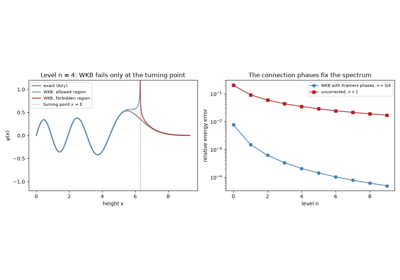
Building on de Broglie’s matter wave, Gregor Wentzel, Hendrik Kramers, and Leon Brillouin – following Harold Jeffreys’ earlier, independent mathematical treatment of the same asymptotic expansion – showed in 1926 how to recover Schrodinger’s exact wave mechanics as a controlled semiclassical limit. Writing the wavefunction as an amplitude times a rapidly oscillating phase,
and expanding order by order in \(\hbar\), the WKB approximation reproduces the classical limit exactly where it should: the amplitude \(p(x)^{-1/2}\) is precisely the classical probability of finding a particle where it moves slowest, and matching the oscillatory solution through each turning point (via the Airy-function connection formulas) costs a phase of \(\pi/4\), refining Wilson-Sommerfeld’s integer quantization into the half-integer Einstein-Brillouin-Keller (EBK) rule.
Implementation: physicskit.semiclassical.core.wkb.classical_momentum()
and turning_points() build the
semiclassical momentum \(p(x)\) and locate its turning points;
wkb_action() and
wkb_wavefunction() assemble
the resulting approximate wavefunction, reproducing the node-counting
theorem and the exact harmonic-oscillator spectrum to machine precision.
References: G. Wentzel, Z. Phys. 38, 518-529 (1926); H. Kramers, Z. Phys. 39, 828-840 (1926); L. Brillouin, C. R. Acad. Sci. 183, 24-26 (1926); precursor H. Jeffreys, Proc. London Math. Soc. 23, 428-436 (1925).
The WKB approximation: connection formulas on the quantum bouncer
1927 – Heisenberg’s Uncertainty Principle#
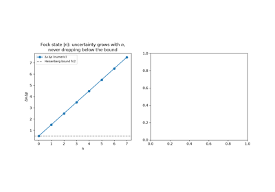
Werner Heisenberg had already given quantum mechanics its first formulation in 1925, replacing classical trajectories with infinite arrays (“matrices”) of transition amplitudes – matrix mechanics, in which position and momentum are non-commuting operators satisfying \([\hat x,\hat p] = i\hbar\). Heisenberg’s initial paper treated only one degree of freedom and left the general algebra incomplete; its full development into a systematic many-body matrix mechanics is jointly credited to Heisenberg, Max Born, and Pascual Jordan, whose “Drei-Manner- Arbeit” (“three-man paper”) supplied the rigorous multi-dimensional formulation, including the canonical commutation relation in the form above. In 1927 Heisenberg drew out that algebra’s starkest physical consequence: position and momentum cannot both be known to arbitrary precision,
This is not a statement about measurement clumsiness but a structural property of any state – a direct consequence of \(x\) and \(p\) failing to commute, and the first hint that quantum mechanics would demand a wholesale revision of what “knowing a system’s state” even means.
Implementation: physicskit.quantum.utils.measure.uncertainty()
computes \(\Delta x\), \(\Delta p\), and their product directly
from a wavefunction, checking the Heisenberg bound;
physicskit.quantum.core.operators.commutator() together with
position_operator() and
momentum_operator() verify the
underlying canonical commutation relation \([\hat x,\hat p]=i\hbar\)
in a truncated oscillator basis.
References: W. Heisenberg, Z. Phys. 33, 879-893 (1925); M. Born and P. Jordan, Z. Phys. 34, 858-888 (1925); M. Born, W. Heisenberg, and P. Jordan, Z. Phys. 35, 557-615 (1926); the uncertainty principle itself, W. Heisenberg, Z. Phys. 43, 172-198 (1927).
1927 – Ehrenfest’s Theorem#
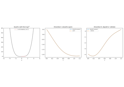
Paul Ehrenfest asked how classical mechanics could ever emerge from a theory built entirely on wavefunctions and operators, and found that it already had: the expectation values of position and momentum obey Newton’s equations of motion exactly, for any potential, not merely a harmonic one,
This is a precise structural fact about the Schrodinger equation, not an approximation valid only for slowly varying potentials – the subtlety is that the second equation involves \(\langle dV/dx\rangle\), the average of the force over the whole spread-out wavefunction, which coincides with the classical force evaluated at the mean position, \(-dV/dx(\langle x\rangle)\), only when \(V\) is quadratic. For any other potential a wavepacket’s centroid drifts away from the corresponding classical trajectory as it spreads, broadens, or splits – the precise sense in which quantum and classical dynamics agree exactly in expectation value, yet disagree about everything a single classical trajectory would predict.
Implementation: physicskit.quantum.core.solvers.SplitOperatorSolver1D
propagates an arbitrary wavepacket through an arbitrary potential, and
physicskit.quantum.utils.measure.ExpectationMonitor records
\(\langle x\rangle(t)\) and \(\langle p\rangle(t)\) from each
snapshot; comparing their numerical time derivatives against
\(\langle p\rangle/m\) and \(-\langle dV/dx\rangle\), computed
independently via expectation_value(),
verifies both Ehrenfest identities directly from a real, propagated
wavefunction in a genuinely anharmonic (quartic) well; the same propagated
frames also feed WignerVisualizer,
showing the state’s phase-space distribution shear away from a rigid
rotation as the anharmonic potential acts, with the \((\langle
x\rangle,\langle p\rangle)\) trajectory traced on top of it.
References: P. Ehrenfest, Z. Phys. 45, 455-457 (1927).
1927 – Dirac’s Time-Dependent Perturbation Theory#
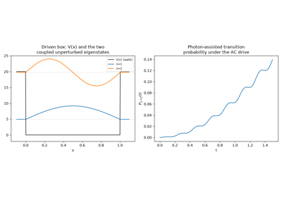
Paul Dirac, developing the quantum theory of radiation, worked out how a weak, time-dependent perturbation drives transitions between the unperturbed stationary states of a system – the foundation of time-dependent perturbation theory. Two decades later Enrico Fermi gave the leading-order transition-rate result a name that stuck: the “golden rule,” so called in his course-derived textbook Nuclear Physics, compiled from his University of Chicago lectures and published in 1950 – not, as sometimes stated, unpublished lecture notes. The same machinery describes a system driven periodically in time, where transitions become resonant multiphoton processes whenever an integer number of drive quanta \(\hbar\omega\) bridges an energy gap.
Implementation: physicskit.quantum.chapters.perturbation.FloquetDrivenBox
propagates a periodically driven infinite well with the FFT split-operator
method, and its
transition_probability()
method exhibits exactly these resonant multiphoton transitions between box
eigenstates.
References: P. A. M. Dirac, Proc. R. Soc. A 114(767), 243-265 (1927); “golden rule” naming, E. Fermi, Nuclear Physics (University of Chicago Press, 1950), a textbook compiled from his lecture course.
Floquet-driven box: time-dependent perturbation theory
1927 – Faxen and Holtsmark: Partial-Wave Analysis#
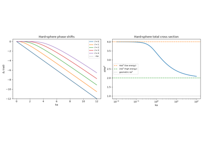
Hilding Faxen and Johan Holtsmark, studying the anomalously low scattering of slow electrons by noble-gas atoms (the Ramsauer-Townsend effect), expanded the scattered wave of a central potential in angular momentum eigenstates. Rotational symmetry means each partial wave \(\ell\) scatters independently, and the potential only changes its phase at large distances by a phase shift \(\delta_\ell\):
Only waves with \(\ell \lesssim ka\) reach a potential of range \(a\), so at low energy a handful of phase shifts describe everything. Two classic consequences: a hard sphere scatters with cross section \(4\pi a^2\) at low energy (four times its geometric area) and \(2\pi a^2\) at high energy (the extra \(\pi a^2\) is the diffraction shadow), and by Levinson’s theorem (1949) the zero-energy phase shift counts the bound states. Phase-shift analysis is still how nuclear and particle scattering data are reported.
Implementation: physicskit.quantum.chapters.scattering.partial_wave_phase_shifts()
computes \(\delta_\ell(k)\) for any short-range potential with
Calogero’s variable-phase equation;
hard_sphere_phase_shifts()
gives the exact hard-sphere result,
born_phase_shifts() their
weak-potential limit, and
partial_wave_amplitude() and
partial_wave_cross_section()
resum the series.
References: H. Faxen and J. Holtsmark, “Beitrag zur Theorie des Durchganges langsamer Elektronen durch Gase,” Z. Phys. 45, 307-324 (1927); F. Calogero, Variable Phase Approach to Potential Scattering (Academic Press, 1967); N. Levinson, Kgl. Danske Videnskab. Selskab, Mat.-fys. Medd. 25, No. 9 (1949).
Partial-wave analysis: phase shifts of the hard sphere and the square well
1928 – The Dirac Equation and the Fine Structure of Hydrogen#
The Klein-Gordon equation, \((\partial_t^2 - \nabla^2 + m^2)\phi = 0\) (\(\hbar = c = 1\)), the obvious relativistic wave equation, had two problems: it is second order in time, so \(|\phi|^2\) is not a conserved probability density, and it has no place for spin. Paul Dirac looked for an equation first order in time and space whose square gives \(E^2 = p^2 + m^2\). This forced the coefficients to be \(4\times4\) matrices obeying \(\{\gamma^\mu,\gamma^\nu\} = 2g^{\mu\nu}\),
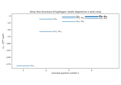
acting on four-component spinors. The equation gave spin 1/2 and the electron’s \(g = 2\) magnetic moment without extra assumptions. Solved for the Coulomb potential (by Darwin and Gordon within the year), it gives hydrogen levels that depend only on \(n\) and \(j\),
reproducing Sommerfeld’s 1916 fine-structure formula. The negative-energy solutions it also predicts led Dirac to the positron (1931), found by Anderson in 1932.
Implementation: physicskit.quantum.chapters.relativistic.dirac_hydrogen_energy()
evaluates the exact Dirac-Coulomb levels and
fine_structure_expansion()
their \((Z\alpha)^4\) expansion;
gamma_matrices(),
dirac_hamiltonian() and
dirac_plane_wave_spinor()
give the free equation and its positive- and negative-energy solutions,
and klein_gordon_dispersion()
and klein_gordon_plane_wave()
the free Klein-Gordon ones.
References: P. A. M. Dirac, “The Quantum Theory of the Electron,” Proc. R. Soc. A 117, 610-624 (1928); C. G. Darwin, Proc. R. Soc. A 118, 654-680 (1928); W. Gordon, Z. Phys. 48, 11-14 (1928); O. Klein, Z. Phys. 37, 895-906 (1926); W. Gordon, Z. Phys. 40, 117-133 (1926).
The Dirac equation and the fine structure of hydrogen
1928 – Gamow, Gurney and Condon: Quantum Tunneling#
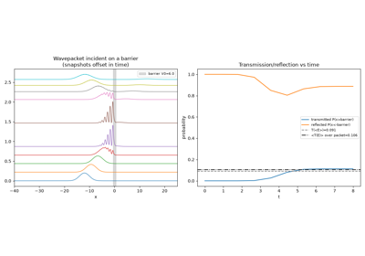
George Gamow, and independently Ronald Gurney and Edward Condon, explained why radioactive nuclei undergo alpha decay at all: classically, the alpha particle sits in a potential well surrounded by a Coulomb barrier far higher than its kinetic energy, and should never escape. Quantum mechanically, the wavefunction does not vanish inside a classically forbidden region – it decays exponentially but remains nonzero – giving a small but nonzero probability of finding the particle on the far side of the barrier. This single idea, quantum tunneling, explained the enormous range of observed alpha-decay half-lives (many orders of magnitude, for barriers differing only modestly in height) and remains the archetypal example of a genuinely quantum phenomenon with no classical counterpart.
Implementation: physicskit.quantum.chapters.potentials.FiniteSquareWell.scattering()
gives the exact transmission probability through a barrier, continuing
correctly into the sub-barrier tunneling regime via complex arithmetic;
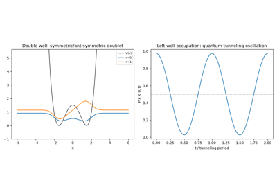
physicskit.quantum.chapters.potentials.DoubleWellSimulator.tunneling_oscillation()
and left_well_probability()
reproduce the related phenomenon of coherent tunneling oscillation between
the two wells of a symmetric double well. Beyond the stationary
transmission coefficient,
wavepacket_scattering()
propagates an actual moving Gaussian wavepacket through the same barrier
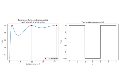
(or, with a positive well depth instead, the related resonant-scattering
case) with the FFT split-operator method, splitting it into a reflected
and a transmitted piece in real time; and
tunneling_wavefunction()
gives the complex two-state wavefunction underlying the density-only
tunneling_oscillation above. Both are rendered frame by frame with
animate_density(). See
the barrier-tunneling animation in
Real-time barrier tunneling, the animated
well-scattering case in
The Ramsauer-Townsend effect, and
the double-well oscillation, including its animated complex-valued version,
in Double-well tunneling.
References: G. Gamow, Z. Phys. 51, 204-212 (1928); R. Gurney and E. Condon, Nature 122, 439 (1928), and Phys. Rev. 33, 127-140 (1929).
1928 – The Van Vleck-Morette Semiclassical Propagator#
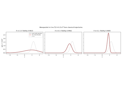
The same semiclassical logic behind WKB applies equally to time evolution rather than stationary states: in 1928 John Van Vleck (extended into a full path-integral formulation by Cecile DeWitt-Morette in 1951) showed that the quantum propagator \(\langle x\rvert e^{-i\hat Ht/\hbar}\lvert x_0\rangle\) is dominated, to leading order in \(\hbar\), by a single classical trajectory connecting \(x_0\) to \(x\) in time \(t\),
where \(S\) is the classical action along that trajectory and \(\sigma\) (the Maslov index) counts the caustics – focal points where nearby trajectories cross – it passes through. This single-trajectory picture of propagation, two decades before Richard Feynman’s 1948 path-integral formulation summed over every trajectory rather than just the classical one, is the direct ancestor of every semiclassical propagation method used in modern quantum chaos and chemical physics.
Implementation: physicskit.semiclassical.core.propagators.propagate_trajectory_monodromy_action()
integrates a classical trajectory together with its monodromy matrix and
action; van_vleck_prefactor(),
count_caustics(), and
van_vleck_propagator_1d()
assemble these into exactly the propagator amplitude above, Maslov phase
included.
References: J. Van Vleck, PNAS 14(2), 178-188 (1928); C. Morette, Phys. Rev. 81, 848-852 (1951); R. P. Feynman, “Space-Time Approach to Non-Relativistic Quantum Mechanics,” Rev. Mod. Phys. 20, 367-387 (1948).
The Van Vleck-Morette propagator beyond quadratic potentials
1929 – Klein’s Paradox#
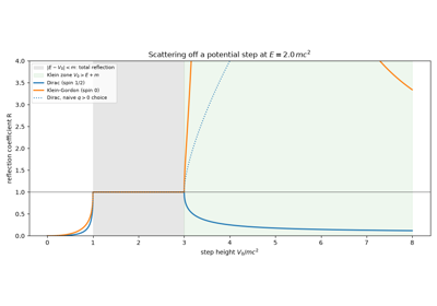
Within a year of Dirac’s equation, Oskar Klein solved it for an electron hitting a potential step \(V_0\). For a step higher than \(E + mc^2\) he found that the electron is partly transmitted, and that the transmission stays finite even as \(V_0 \to \infty\), in contrast to non-relativistic quantum mechanics, where a tall barrier reflects almost everything. Matching Dirac spinors at the step gives
The explanation, which took decades to settle, is that the step lowers the negative-energy (antiparticle) continuum to the electron’s energy: the transmitted wave is a positron, and the step creates electron-positron pairs. Choosing the transmitted momentum by its group velocity makes \(0 < R < 1\) for fermions, while spin-0 Klein-Gordon particles have \(R > 1\) (bosonic “superradiance”). Klein tunneling has been observed in graphene, whose electrons obey a massless Dirac equation.
Implementation: physicskit.quantum.chapters.relativistic.dirac_step_scattering()
and klein_gordon_step_scattering()
give \(R\) and \(T\) for all step heights, with either choice of
the transmitted momentum’s sign.
References: O. Klein, “Die Reflexion von Elektronen an einem Potentialsprung nach der relativistischen Dynamik von Dirac,” Z. Phys. 53, 157-165 (1929); N. Dombey and A. Calogeracos, “Seventy years of the Klein paradox,” Phys. Rep. 315, 41-58 (1999); M. I. Katsnelson, K. S. Novoselov, and A. K. Geim, Nature Phys. 2, 620-625 (2006).
Klein’s paradox: relativistic particles at a tall potential step
1928-1930 – Hartree and Fock: The Self-Consistent Field#
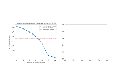
The Schrodinger equation for \(N\) interacting electrons lives in \(3N\) dimensions and cannot be solved directly for anything beyond the smallest atoms. Douglas Hartree proposed in 1928 that each electron moves in the average electrostatic field of the nucleus and all the other electrons, and that this field be computed from the electrons’ own orbitals and iterated until it reproduces itself: a self-consistent field. Vladimir Fock and John Slater (1930) showed that writing the wavefunction as an antisymmetrized product, a Slater determinant, adds an exchange term with no classical analogue. The best single determinant satisfies the Hartree-Fock equations; expanding the orbitals in a finite basis turns them into the matrix Roothaan-Hall equations (1951),
solved iteratively. Hartree-Fock recovers over 99% of an atom’s total energy; the small remainder, the correlation energy, is what later methods of quantum chemistry set out to compute.
Implementation: physicskit.quantum.chapters.hartree_fock.restricted_hartree_fock()
runs the closed-shell Roothaan SCF procedure with the closed-form Gaussian
integrals of overlap_matrix(),
kinetic_matrix(),
nuclear_attraction_matrix(),
and electron_repulsion_tensor(),
in STO-3G (sto3g_1s()) or
even-tempered (even_tempered_s_basis())
s bases. It reproduces Szabo and Ostlund’s textbook results for
\(\mathrm H_2\) and \(\mathrm{HeH^+}\) and the helium Hartree-Fock
limit.
References: D. R. Hartree, “The Wave Mechanics of an Atom with a Non-Coulomb Central Field,” Proc. Camb. Phil. Soc. 24, 89-110 (1928); V. Fock, “Naherungsmethode zur Losung des quantenmechanischen Mehrkorperproblems,” Z. Phys. 61, 126-148 (1930); J. C. Slater, Phys. Rev. 35, 210-211 (1930); C. C. J. Roothaan, Rev. Mod. Phys. 23, 69-89 (1951); A. Szabo and N. S. Ostlund, Modern Quantum Chemistry (1989), Ch. 3.
Hartree-Fock: the self-consistent field for H₂ and helium
1930 – Dirac’s Operator Method and the Harmonic Oscillator#
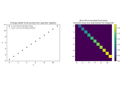
In The Principles of Quantum Mechanics (1930), Dirac popularized an algebraic shortcut for the quantum harmonic oscillator that sidesteps solving the Schrodinger equation as a differential equation entirely: factor the Hamiltonian into raising and lowering (“ladder”) operators \(\hat a^\dagger, \hat a\) satisfying \([\hat a,\hat a^\dagger]=1\), build the entire spectrum by repeated raising from a ground state annihilated by \(\hat a\), and read off \(E_n=\hbar\omega(n+\tfrac12)\) directly from the operator algebra. The technique, generalized to Glauber’s 1963 coherent states \(\lvert\alpha\rangle\) – eigenstates of \(\hat a\) that behave as classically as a quantum state can – became the standard language of quantum optics.
Implementation: physicskit.quantum.core.operators.annihilation_operator(),
creation_operator(), and
number_operator() build exactly
this ladder-operator algebra in a truncated Fock basis;
physicskit.quantum.chapters.harmonic_spin.HarmonicOscillator.coherent_wavefunction()
and squeezed_vacuum_wavefunction()
build Glauber coherent states and their squeezed generalizations from this
same Fock-state expansion. The coherent/squeezed states are shown in
The harmonic oscillator suite.
References: P. A. M. Dirac, The Principles of Quantum Mechanics (Clarendon Press, 1930); coherent states, R. Glauber, Phys. Rev. 131, 2766-2788 (1963).
1935 – The EPR Paradox#
Einstein, Podolsky, and Rosen argued, in a paper meant to demonstrate quantum mechanics’ incompleteness, that if two particles are prepared in a correlated (“entangled”) state and then separated by an arbitrary distance, measuring one instantaneously determines the corresponding outcome for the other. Since no real influence should propagate faster than light, EPR concluded that the particles must have possessed definite values all along, carried by some “hidden variable” quantum mechanics simply fails to describe – entanglement, to them, was evidence the theory was unfinished rather than a genuinely new feature of nature. It would take Bell twenty-nine years to show that this intuition, however reasonable, is testable – and wrong.
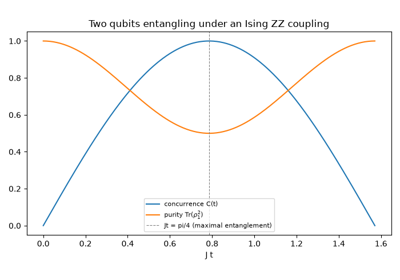
Implementation: physicskit.quantum.chapters.entanglement.IsingEntangler
builds exactly the kind of correlated two-particle state EPR had in mind,
but shows how it actually arises rather than simply positing it: two
qubits, each individually unbiased and initially unentangled
(\(\lvert+\rangle\otimes\lvert+\rangle\)), accumulate genuine
entanglement purely through an Ising coupling
\(\hat H=\hbar J\,\sigma_z^{(1)}\otimes\sigma_z^{(2)}\), with its
concurrence()
and purity()
methods tracking the buildup from a product state (concurrence 0) to a
maximally entangled, Bell-equivalent state (concurrence 1) at
\(Jt=\pi/4\), animated with
animate_entanglement_growth().
See it in
Dynamical entanglement generation.
References: A. Einstein, B. Podolsky, and N. Rosen, Phys. Rev. 47, 777-780 (1935).
1935 – Schrodinger Names “Entanglement”#
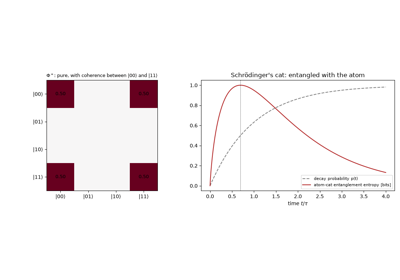
Responding directly to Einstein, Podolsky, and Rosen within months of their paper, Erwin Schrodinger wrote a long analysis of what their correlated state actually implies, and in it coined the word that has described the phenomenon ever since: Verschrankung, “entanglement.” Schrodinger argued that entanglement – not any single particle’s uncertainty – is the truly characteristic trait of quantum mechanics, the feature that most sharply separates it from any classical theory, and in the same paper introduced his now-famous cat, whose life hangs on the entangled fate of a radioactive atom, to dramatize how strange it is that this feature seems to survive all the way up to macroscopic scale. The package’s own entanglement measures and Bell-state machinery are built on precisely the concept Schrodinger named here, three decades before Bell showed it was testable and half a century before it acquired experimental and technological weight of its own.
Connection: physicskit.quantum.chapters.entanglement.IsingEntangler
and physicskit.quantum.chapters.entanglement.bell_state(), together
with the concurrence and purity measures used throughout the entanglement
entries in this chronology, quantify exactly the non-classical
correlation – entanglement – that Schrodinger’s paper first named and
argued was quantum mechanics’ defining feature.
References: E. Schrodinger, “Die gegenwartige Situation in der Quantenmechanik,” Naturwissenschaften 23, 807-812, 823-828, 844-849 (1935); English translation, “The Present Situation in Quantum Mechanics,” Proc. Am. Phil. Soc. 124, 323-338 (1980).
Schrödinger names entanglement: the whole known, the parts not
1937-1946 – Rabi’s Magnetic Resonance Method and the Bloch Sphere#
In 1937, at Columbia University, Isidor Rabi devised the molecular-beam magnetic-resonance method: a beam of molecules passes through a static magnetic field and a region of oscillating field tuned near the natural (Larmor) precession frequency of the nuclear magnetic moment, and that moment’s projection flips with near-unit probability exactly when the drive is resonant – the phenomenon now called a “Rabi oscillation.” The theoretical paper was completed in February and published in April 1937; the first experimental resonance curve, obtained with a lithium chloride beam, was submitted to Physical Review in January 1938. The method gave, for the first time, a direct and extraordinarily precise measurement of nuclear magnetic moments, and Rabi received the 1944 Nobel Prize in Physics for it.
Nine years later, at Stanford, Felix Bloch (and independently, at Harvard, Edward Purcell) extended the same resonance idea from a molecular beam in vacuum to nuclear spins in bulk matter, detecting the induced radiofrequency signal directly rather than a deflected beam – “nuclear induction,” published in 1946. In that same paper Bloch introduced the geometric device that now carries his name: representing bulk nuclear magnetization as a classical vector precessing (under a static field) or nutating (under a resonant drive) on the surface of a unit sphere, exactly as a classical magnetic moment would. Bloch’s own sphere was a picture of a real classical vector – an ensemble average over many nuclear spins – rather than the quantum state of one two-level system; the now-standard generalization of the same geometric picture to the pure quantum state of any single two-level system (a single spin, or, in modern usage, a single qubit) is usually credited to a 1957 paper by Richard Feynman, Frank Vernon Jr., and Robert Hellwarth, which showed that any two-state Schrodinger evolution can be mapped onto exactly Bloch’s precession/nutation geometry. Bloch and Purcell shared the 1952 Nobel Prize in Physics for the original discovery, the direct ancestor of nuclear magnetic resonance (NMR) spectroscopy, MRI, and – via the Feynman-Vernon-Hellwarth generalization – the standard way of visualizing a single qubit’s state in modern quantum computing.
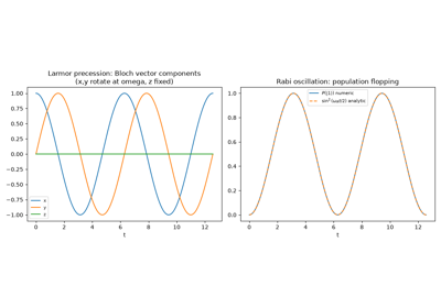
the closed-form rotating-wave-approximation propagator for a two-level system driven near resonance – the “Rabi formula” – with \(\Delta\) the drive detuning and \(\Omega\) the drive strength.
Implementation: physicskit.quantum.chapters.spin.RabiProblem
implements exactly this closed-form propagator, and its
excited_state_population()
method reproduces the Rabi formula’s population-flopping curve;
state_to_bloch_trajectory()
and animate_bloch_sphere()
trace the resulting state as a vector precessing/nutating on Bloch’s own
sphere, animated frame by frame with a matplotlib FuncAnimation. See the
Rabi-driven Bloch-sphere animation in
Rabi’s magnetic resonance on the Bloch sphere.
References: I. Rabi, Phys. Rev. 51, 652-654 (1937); I. Rabi et al., Phys. Rev. 53, 318 (1938); F. Bloch, Phys. Rev. 70, 460-474 (1946); E. M. Purcell, H. C. Torrey, and R. V. Pound, Phys. Rev. 69, 37-38 (1946); generalization of the Bloch sphere to a single two-state quantum system, R. P. Feynman, F. L. Vernon Jr., and R. W. Hellwarth, J. Appl. Phys. 28, 49-52 (1957).
1959 – The Aharonov-Bohm Effect#
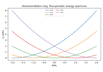
Yakir Aharonov and David Bohm predicted, in 1959, a startling consequence of quantum mechanics with no classical analogue at all: a charged particle can be measurably affected by an electromagnetic potential even in a region where every field it could classically feel – \(\mathbf B\) and \(\mathbf E\) – vanishes identically. Threading a magnetic flux \(\Phi\) through the hole of a conducting ring, without ever letting the electron enter the field region, shifts every energy level of the ring,
purely through the vector potential’s Aharonov-Bohm phase \(\Delta\phi = 2\pi\Phi/\Phi_0\) picked up by the electron’s wavefunction as it circles the ring. Confirmed experimentally by Akira Tonomura’s group using electron holography in 1986, the effect showed that the electromagnetic potentials – not just the fields derived from them – are physically real, and it seeded the entire field of mesoscopic persistent-current physics. The same phase effect had in fact been derived a decade earlier, in 1949, by Werner Ehrenberg and Raymond Siday, who noted it explicitly in a paper on electron optics that went largely unnoticed at the time; in recognition of that priority the effect is sometimes called the “Ehrenberg-Siday-Aharonov-Bohm effect.”
Implementation: physicskit.quantum.chapters.entanglement.AharonovBohmRing
reproduces exactly this flux-dependent spectrum in its energy and
spectrum methods, its aharonov_bohm_phase method gives
\(\Delta\phi\), and its persistent_current method computes the
equilibrium ring current the flux dependence implies.
References: Y. Aharonov and D. Bohm, Phys. Rev. 115, 485-491 (1959); experimental confirmation, A. Tonomura et al., Phys. Rev. Lett. 56, 792-795 (1986); priority, W. Ehrenberg and R. E. Siday, Proc. Phys. Soc. B 62, 8-21 (1949).
1961 – Jonsson’s Electron Double-Slit Experiment#
Richard Feynman would later call the electron double-slit experiment “a phenomenon which is impossible … to explain in any classical way, and which has in it the heart of quantum mechanics.” Claus Jonsson had already performed it: using electron-biprism interferometry through up to five parallel micro-slits machined in copper foil, he observed exactly the interference fringes de Broglie’s matter waves and Born’s probabilistic interpretation predicted, extending Young’s 1801 two-slit demonstration for light to individual massive particles for the first time. In 2002, readers of Physics World voted the electron double-slit experiment “the most beautiful experiment in physics.”
the same two-amplitude interference law as classical wave optics, now describing the probability density of finding a single electron – fired one at a time – at position \(y\) on the downstream screen.
Implementation: physicskit.quantum.chapters.wave_packets.TwinSlit
builds this two-source interference pattern from coherent Gaussian slit
sources propagated to a screen; its amplitude and intensity
methods reproduce the fringe pattern \(\lvert\psi_1+\psi_2\rvert^2\)
directly. See it in Jönsson’s electron double slit: interference one electron at a time.
Rather than that far-field (Fraunhofer) shortcut,
double_slit_potential() and
propagate_double_slit()
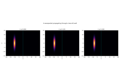
build the same two-gap wall as a genuine 2D potential and propagate a
Gaussian wavepacket through it with
SplitOperatorSolver2D, so the
fringe pattern builds up frame by frame from the full time-dependent
Schrodinger equation rather than a closed-form formula, animated with
animate_density_2d().
See it in
The double-slit experiment, propagated in time.
References: C. Jonsson, Z. Phys. 161, 454-474 (1961); English translation, Am. J. Phys. 42, 4-11 (1974).
Jönsson’s electron double slit: interference one electron at a time
1964 – Bell’s Theorem and the CHSH Inequality#
John Bell showed that any theory of the EPR type – one where measurement outcomes are fixed in advance by local “hidden variables,” unknown to quantum mechanics but real nonetheless – must satisfy an inequality that quantum mechanics itself predicts will be violated. Clauser, Horne, Shimony, and Holt reformulated Bell’s inequality in 1969 into the experimentally practical CHSH form,
which the singlet state violates up to the Tsirelson bound \(\lvert S\rvert = 2\sqrt2 \approx 2.828\), established by Boris Tsirelson in 1980 as quantum mechanics’ own ceiling. Experiments – from Aspect’s in the early 1980s to the loophole-free tests of 2015 – have consistently confirmed the quantum prediction, closing the question EPR opened: entanglement is real, and no local hidden-variable theory can reproduce it.
Implementation: physicskit.quantum.chapters.entanglement.bell_state()
builds the singlet used throughout;
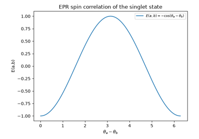
BellCorrelations computes
the spin correlation(),
and its
chsh_S()
and chsh_optimal()
methods reproduce exactly this CHSH violation up to the Tsirelson bound.
References: J. Bell, Physics 1(3), 195-200 (1964); J. Clauser, M. Horne, A. Shimony, and R. Holt, Phys. Rev. Lett. 23, 880-884 (1969); B. Tsirelson, Lett. Math. Phys. 4, 93-100 (1980); A. Aspect et al., Phys. Rev. Lett. 49, 1804-1807 (1982); loophole-free tests, B. Hensen et al., Nature 526, 682-686 (2015).
1971 – Gutzwiller’s Trace Formula#
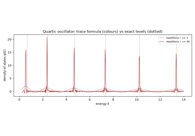
Martin Gutzwiller asked, in a series of papers culminating in 1971, how a quantum energy spectrum could be reconstructed purely from the classical mechanics of a system – including chaotic systems, with no exact quantum numbers at all. His answer, the trace formula, expresses the quantum density of states as a sum over every classical periodic orbit, weighted by that orbit’s action, period, and (in higher dimensions) stability:
where the outer sum runs over each primitive periodic orbit \(p\) (action \(S_p\), period \(T_p\), monodromy matrix \(M_p\), Maslov index \(\sigma_p\)) and the inner sum over its repetitions \(r\). For an integrable one-dimensional system this identity is exact rather than approximate, and it founded the field of quantum chaos: the first rigorous bridge between a system’s classical dynamics – regular or chaotic – and the fine structure of its quantum spectrum.
Implementation: physicskit.semiclassical.core.gutzwiller.classical_period()
supplies \(T(E)=dS/dE\) for a 1D bound orbit, and
gutzwiller_density_of_states()
sums the resulting exact 1D trace formula, reconstructing the
Bohr-Sommerfeld spectrum’s delta-function peaks purely from repetitions
of a single classical orbit;
gutzwiller_amplitude_from_monodromy()
gives the general stability amplitude \(1/\sqrt{\lvert
2-\operatorname{tr}M\rvert}\) needed beyond the exactly-solvable 1D case.
References: M. Gutzwiller, J. Math. Phys. 12, 343-358 (1971).
Gutzwiller’s trace formula: a spectrum from classical orbits
1976 – Lindblad’s Master Equation for Open Quantum Systems#
No real quantum system is perfectly isolated: an atom radiates into the electromagnetic vacuum, a superconducting qubit leaks energy into its circuit, and every such coupling turns pure states into mixed ones. Goran Lindblad, and simultaneously Vittorio Gorini, Andrzej Kossakowski and George Sudarshan, answered the structural question of what equations of motion are even allowed for the density matrix of a system whose environment has no memory. Requiring the evolution to be a semigroup of completely positive, trace-preserving maps – so that probabilities stay probabilities even when the system is entangled with something else – forces the unique form
with one “jump” operator \(L_k\) per dissipative channel. For a qubit, spontaneous decay \(L = \sqrt{1/T_1}\,\sigma_-\) and pure dephasing \(L \propto \sigma_z\) reproduce exactly the phenomenological relaxation times \(T_1\) and \(T_2\) that Felix Bloch had written down for nuclear magnetic resonance thirty years earlier, now on a rigorous quantum footing. The GKSL equation is today the working model of decoherence in quantum optics and quantum computing.
Implementation: physicskit.quantum.chapters.open_systems.solve_lindblad()
propagates \(\rho(t)\) exactly via the matrix exponential of the
Liouvillian built by
lindblad_superoperator();
t1_t2_collapse_operators()
builds the collapse operators for given \(T_1\) and \(T_2\),
lindblad_steady_state()
finds the stationary state, and
amplitude_damping_kraus()
and dephasing_kraus() give
the equivalent finite-time quantum channels.
References: G. Lindblad, “On the generators of quantum dynamical semigroups,” Commun. Math. Phys. 48, 119-130 (1976); V. Gorini, A. Kossakowski, and E. C. G. Sudarshan, J. Math. Phys. 17, 821-825 (1976).
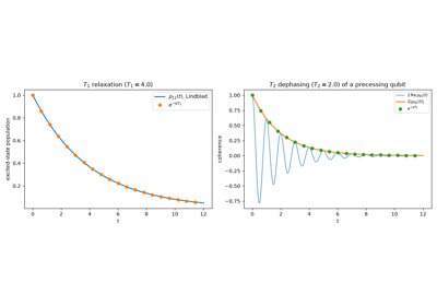
The Lindblad master equation: T1 relaxation and T2 dephasing
1982 – The No-Cloning Theorem#
William Wootters and Wojciech Zurek, and independently Dennis Dieks, proved a negative result as consequential as any of Bell’s: no unitary process can take an arbitrary, unknown quantum state and produce two independent copies of it, \(\lvert\psi\rangle\lvert e\rangle \mapsto \lvert\psi\rangle\lvert\psi\rangle\), for every \(\lvert\psi\rangle\) simultaneously. The proof is a direct consequence of the linearity that makes quantum mechanics quantum mechanics: a fixed unitary that faithfully clones two particular non-orthogonal states \(\lvert\psi\rangle\) and \(\lvert\phi\rangle\) would, by linearity, act on their superposition in a way that is not a faithful copy of that superposition – a contradiction unless the two states were orthogonal (or identical) to begin with. The no-cloning theorem is the reason quantum cryptography can detect eavesdropping (an eavesdropper cannot covertly copy a qubit to inspect it later), and the reason quantum error correction has to encode information redundantly across entangled qubits rather than by simply duplicating a single qubit’s state.
Connection: the package has no dedicated cloning-machine example, but
the two-qubit unitary machinery the theorem constrains is exactly the
machinery built elsewhere in this chronology:
physicskit.quantum.chapters.entanglement.bell_state() and
IsingEntangler both
construct genuinely entangled two-qubit states from unitary, linear time
evolution, the same linearity whose consequences the Wootters-Zurek-Dieks
proof exploits; no combination of a fixed unitary and an ancilla built
from these same primitives could instead be made to duplicate an arbitrary
input qubit.
References: W. K. Wootters and W. H. Zurek, Nature 299, 802-803 (1982); D. Dieks, Phys. Lett. A 92, 271-272 (1982).
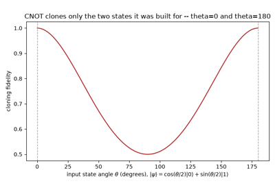
The no-cloning theorem: why a fixed unitary can copy a basis, not a state
1984 – Heller’s Quantum Scars and the Herman-Kluk Propagator#
Eric Heller discovered, in 1984, a phenomenon that contradicted the prevailing expectation for quantum systems whose classical dynamics is chaotic: rather than spreading uniformly over all of accessible phase space (as random-matrix “quantum ergodicity” predicted they should), many eigenstates of chaotic billiards show statistically significant density enhancement concentrated along a handful of short, unstable periodic orbits – “scars.” That same year, Michael Herman and Edward Kluk jointly published, as co-authors of a single paper, a multi-trajectory semiclassical propagator that made computing such wavepacket dynamics in chaotic and anharmonic systems tractable, replacing the single (and often singular, at a caustic) Van Vleck trajectory with a smooth sum over a whole family of frozen Gaussian wavepackets,
an integral over classical initial conditions that, unlike the single Van Vleck trajectory, never itself passes through a caustic singularity.
Implementation: physicskit.semiclassical.systems.scarring.bouncing_ball_energies()
and bouncing_ball_orbit_points()
locate the stadium billiard’s shortest unstable periodic orbit family, and
scar_enhancement()
quantifies exactly Heller’s density-enhancement signature, \(\eta =
\langle\lvert\psi\rvert^2\rangle_{\text{tube}}/\langle\lvert\psi\rvert^2\rangle_{\text{billiard}}\);
herman_kluk_propagate_wavepacket(),
built on frozen_gaussian_1d()
and herman_kluk_prefactor(),
implements the Herman-Kluk multi-trajectory propagator above.
References: E. Heller, Phys. Rev. Lett. 53, 1515-1518 (1984); M. Herman and E. Kluk, Chem. Phys. 91, 27-34 (1984) (a single joint paper, not two independent discoveries).
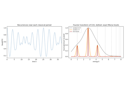
Heller and Herman-Kluk (1984): spectra from wavepacket recurrences
1985 – 1992 – Deutsch, Jozsa, and the First Quantum Algorithm#
Richard Feynman (1982) had argued that only a quantum machine could simulate quantum physics efficiently. David Deutsch (1985) defined the universal quantum computer and gave the first task it does better than any classical machine: deciding with one query whether a one-bit function is constant or balanced. With Richard Jozsa (1992) he extended this to \(n\) bits. Given the promise that \(f:\{0,1\}^n \to \{0,1\}\) is either constant or balanced, a deterministic classical algorithm may need \(2^{n-1} + 1\) evaluations, while one call to the phase oracle \(O_f|x\rangle = (-1)^{f(x)}|x\rangle\), sandwiched between Hadamard layers, suffices:
The superposition queries every input at once, but only the interference between the answers is read out. That pattern of parallel evaluation followed by global interference is shared by every later quantum algorithm.
Implementation: physicskit.quantum.chapters.quantum_circuits.QuantumCircuit
is a state-vector simulator (gates as tensor contractions on a
\((2,)^n\) array), and
deutsch_jozsa_circuit()
builds the algorithm for any truth table.
References: R. P. Feynman, Int. J. Theor. Phys. 21, 467-488 (1982); D. Deutsch, Proc. R. Soc. A 400, 97-117 (1985); D. Deutsch and R. Jozsa, Proc. R. Soc. A 439, 553-558 (1992); R. Cleve, A. Ekert, C. Macchiavello and M. Mosca, Proc. R. Soc. A 454, 339-354 (1998).
The Deutsch-Jozsa algorithm: the first exponential quantum speed-up
1986-1990 – Wave-Packet Revivals#
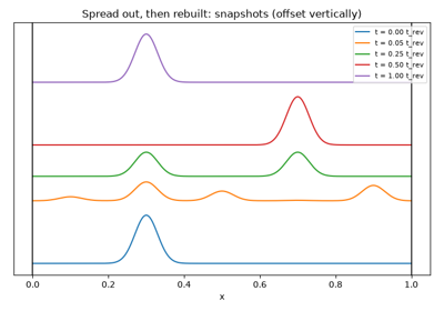
A wavepacket built from many eigenstates of an anharmonic potential – where, unlike the harmonic oscillator, the energy levels are not evenly spaced – spreads and appears to lose all resemblance to its initial shape within a few classical periods. J. Parker and C. R. Stroud predicted theoretically in 1986, and J. A. Yeazell, M. Mallalieu, and C. R. Stroud confirmed experimentally in Rydberg wave packets in 1990, what the quadratic term in the level spacing actually implies: the packet is not gone, only dephased, and it exactly reconstructs itself at a calculable revival time, with smaller-scale “fractional revival” clones (named and analyzed by Ilya Averbukh and Nathan Perelman in 1989) appearing at rational fractions of that time along the way. For the textbook case of a particle in an infinite square well, where \(E_n \propto n^2\) exactly,
and a mirror-image replica of the initial packet appears already at \(t_\text{rev}/2\).
Implementation: physicskit.quantum.chapters.wave_packets.QuantumRevival
expands an arbitrary localized initial state (via gaussian_initial_state
and eigenbasis_coefficients) in the infinite-well eigenbasis and
evolves it with wavefunction; its revival_time property gives
\(t_\text{rev}\) above, and fidelity_to_initial tracks the
wavepacket’s overlap with \(\psi(x,0)\) collapsing and then sharply
recovering at that time. See it in
Wave-packet revivals in the infinite square well.
References: J. Parker and C. Stroud, Phys. Rev. Lett. 56, 716-719 (1986); J. A. Yeazell, M. Mallalieu, and C. R. Stroud Jr., Phys. Rev. Lett. 64, 2007-2010 (1990); fractional revivals, I. Sh. Averbukh and N. F. Perelman, Phys. Lett. A 139, 449-453 (1989).
1992 – Dalibard, Castin, and Molmer: Quantum Trajectories#
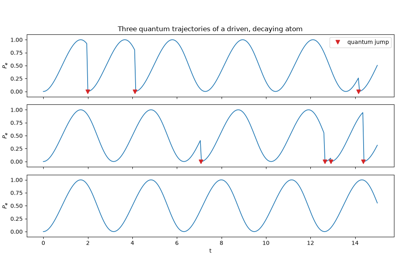
By the late 1980s experiments were watching single trapped ions switch abruptly between bright and dark states – “quantum jumps” that a density matrix, describing only ensemble averages, cannot display. Jean Dalibard, Yvan Castin and Klaus Molmer (and, independently, Dum, Zoller and Ritsch, and Carmichael, who coined the term “quantum trajectories”) showed that the Lindblad equation can be unravelled into stochastic pure-state histories. Between jumps a state evolves under the non-Hermitian effective Hamiltonian
whose shrinking norm is the probability that no jump has yet occurred; at random times a jump \(\psi \to L_k\psi\) is applied. Averaging \(|\psi\rangle\langle\psi|\) over many such trajectories recovers \(\rho(t)\) exactly. Besides giving a picture of what a single photodetected atom does, the method only needs state vectors of dimension \(d\) instead of density matrices of dimension \(d^2\), which is why it is widely used for simulating large open quantum systems.
Implementation: physicskit.quantum.chapters.open_systems.QuantumTrajectories
runs a vectorized ensemble of trajectories with the waiting-time jump
rule, returning a
TrajectoryResult whose
density_matrices average converges to
solve_lindblad()’s
solution and whose jump_times record each trajectory’s photon
emissions.
References: J. Dalibard, Y. Castin, and K. Molmer, “Wave-function approach to dissipative processes in quantum optics,” Phys. Rev. Lett. 68, 580-583 (1992); R. Dum, P. Zoller, and H. Ritsch, Phys. Rev. A 45, 4879-4887 (1992); H. J. Carmichael, An Open Systems Approach to Quantum Optics (Springer, 1993); review: M. B. Plenio and P. L. Knight, Rev. Mod. Phys. 70, 101-144 (1998).
Quantum trajectories: the Monte Carlo wavefunction method
1992 – 2004 – DMRG, Matrix Product States, and Vidal’s TEBD#
The Hilbert space of \(N\) spins has \(2^N\) dimensions, which limits exact diagonalization to a few dozen sites. Steven White’s density matrix renormalization group (1992) found ground states of 1D chains to nearly machine precision by keeping, at each cut of the chain, only the \(\chi\) most important Schmidt states. Östlund and Rommer (1995) recognized that DMRG optimizes a matrix product state,
whose bond dimension \(\chi\) bounds the entanglement entropy across each cut by \(\ln\chi\). Ground states of gapped 1D Hamiltonians obey such an area law (Hastings 2007), so they fit. Guifré Vidal (2003, 2004) turned this into a time-evolution algorithm, time-evolving block decimation (TEBD): a Trotter splitting of \(e^{-iH\delta t}\) into two-site gates on even and odd bonds, each followed by an SVD that truncates the bond back to \(\chi\). In imaginary time it projects onto the ground state. TEBD and its descendants now simulate quenches, transport and finite temperature in chains of hundreds of sites, and the same tensor-network language describes topological order and holographic codes.
Implementation: physicskit.quantum.chapters.tensor_networks.MPS
stores a right-canonical MPS with the Schmidt values of every bond, and
tebd() evolves it in real
or imaginary time under the bond Hamiltonians of
xxz_bond_hamiltonians()
and tfim_bond_hamiltonians(),
which match the exact diagonalization of
physicskit.condensed.spin_chains term by term.
References: S. R. White, Phys. Rev. Lett. 69, 2863-2866 (1992); S. Östlund and S. Rommer, Phys. Rev. Lett. 75, 3537-3540 (1995); G. Vidal, Phys. Rev. Lett. 91, 147902 (2003) and 93, 040502 (2004); U. Schollwöck, Ann. Phys. 326, 96-192 (2011).
TEBD on matrix product states: spin chains beyond exact diagonalization
1994 – Shor’s Algorithm and the Quantum Fourier Transform#
Peter Shor showed that a quantum computer could factor an \(L\)-bit integer in time polynomial in \(L\), while the best known classical algorithms take time exponential in \(L^{1/3}\); the security of RSA rests on that gap. Factoring \(N\) reduces to finding the period \(r\) of \(a^x \bmod N\), since then \(\gcd(a^{r/2} \pm 1, N)\) are usually factors. A register in the superposition \(\sum_x |x\rangle|a^x \bmod N\rangle\) holds the period in its amplitudes, and the quantum Fourier transform
concentrates it into peaks at multiples of \(2^t/r\). Don Coppersmith (1994) built the transform from \(t(t+1)/2\) Hadamard and controlled-phase gates, exponentially fewer operations than the classical fast Fourier transform on the same \(2^t\) amplitudes. A continued-fraction expansion of the measured \(y/2^t\) then gives \(r\). The algorithm started the field of quantum computing as a practical enterprise, and \(15 = 3 \times 5\) was factored on an NMR quantum computer in 2001.
Implementation: physicskit.quantum.chapters.quantum_circuits.qft_circuit()
builds the transform, which equals the DFT matrix to machine precision;
modular_exponentiation_circuit()
prepares the period-finding state (with the modular arithmetic as one
reversible permutation gate), and
shor_period_from_measurement()
recovers \(r\) by continued fractions.
References: P. W. Shor, in Proc. 35th Annual Symposium on Foundations of Computer Science, 124-134 (IEEE, 1994), and SIAM J. Comput. 26, 1484-1509 (1997); D. Coppersmith, IBM Research Report RC19642 (1994); L. M. K. Vandersypen et al., Nature 414, 883-887 (2001).
Shor’s period finding and the quantum Fourier transform
1996 – Grover’s Quantum Search#
Lov Grover found a quantum algorithm that finds one of \(M\) marked items among \(N\) unsorted ones with about \(\tfrac{\pi}{4}\sqrt{N/M}\) oracle queries, where a classical search needs \(O(N/M)\). Bennett, Bernstein, Brassard and Vazirani had shown that no quantum algorithm can do better, so the square-root speed-up is optimal. Starting from the uniform superposition \(|s\rangle\), each iteration applies the oracle, which flips the sign of marked items, and the diffusion operator \(2|s\rangle\langle s| - I\). The two reflections compose to a rotation by \(2\theta\) in the plane of \(|s\rangle\) and the marked state, with \(\sin\theta = \sqrt{M/N}\), so after \(k\) iterations
Going past the optimum rotates the state away again. Generalized as amplitude amplification, the idea speeds up any classical search heuristic quadratically.
Implementation: physicskit.quantum.chapters.quantum_circuits.grover_circuit()
builds the search for any set of marked items, and
grover_success_probability()
and grover_optimal_iterations()
give the rotation formula and the optimal number of iterations.
References: L. K. Grover, in Proc. 28th Annual ACM Symposium on Theory of Computing, 212-219 (1996), and Phys. Rev. Lett. 79, 325-328 (1997); C. H. Bennett, E. Bernstein, G. Brassard and U. Vazirani, SIAM J. Comput. 26, 1510-1523 (1997); M. Boyer, G. Brassard, P. Høyer and A. Tapp, Fortsch. Phys. 46, 493-505 (1998).