Friis’s effective aperture: gain and area (1946)

Friis first wrote his transmission formula not with gains but with the antennas’ effective areas: \(P_r/P_t = A_t A_r/(d\lambda)^2\). A receiving antenna collects the power falling on its effective area \(A_e\), and reciprocity ties that area to its gain, \(A_e = G\lambda^2/4\pi\) (effective_aperture()). 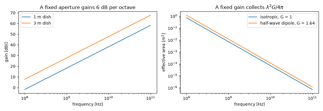For a dish of physical area \(A\) and aperture efficiency \(\eta_a\), \(G = 4\pi\eta_a A/\lambda^2\) (aperture_gain()). A dish of fixed size gains 6 dB at every doubling of frequency, while an antenna of fixed gain collects less and less power.

import matplotlib.pyplot as plt
import numpy as np

from engineeringkit.communications import aperture_gain, db, effective_aperture, friis_received_power, wavelength

The area form and the gain form agree

f, d = 12e9, 36_000e3  # Ku-band, geostationary distance
dish_t, dish_r = np.pi * 1.2**2, np.pi * 0.3**2  # 2.4 m uplink dish, 60 cm TV dish
Gt, Gr = aperture_gain(dish_t, f, 0.65), aperture_gain(dish_r, f, 0.65)
by_area = effective_aperture(Gt, f) * effective_aperture(Gr, f) / (d * wavelength(f)) ** 2
by_gain = friis_received_power(1.0, Gt, Gr, d, f)
print(f"dish gains {float(db(Gt)):.1f} and {float(db(Gr)):.1f} dBi; Pr/Pt = {float(db(by_gain)):.1f} dB")
assert np.isclose(by_area, by_gain)
assert np.isclose(effective_aperture(Gr, f), 0.65 * dish_r)

dish gains 47.7 and 35.7 dBi; Pr/Pt = -121.8 dB

Fixed area versus fixed gain

freqs = np.logspace(8, 11, 61)
fig, axes = plt.subplots(1, 2, figsize=(11, 3.8))
axes[0].semilogx(freqs, db(aperture_gain(np.pi * 0.5**2, freqs, 0.6)), label="1 m dish")
axes[0].semilogx(freqs, db(aperture_gain(np.pi * 1.5**2, freqs, 0.6)), label="3 m dish")
axes[0].set(xlabel="frequency [Hz]", ylabel="gain [dBi]", title="A fixed aperture gains 6 dB per octave")
axes[0].legend()
axes[1].loglog(freqs, effective_aperture(1.0, freqs), label="isotropic, G = 1")
axes[1].loglog(freqs, effective_aperture(1.64, freqs), label="half-wave dipole, G = 1.64")
axes[1].set(xlabel="frequency [Hz]", ylabel="effective area [m$^2$]", title=r"A fixed gain collects $\lambda^2 G/4\pi$")
axes[1].legend()
fig.tight_layout()
ratio = aperture_gain(1.0, 2 * f) / aperture_gain(1.0, f)
assert np.isclose(float(db(ratio)), 6.0206, atol=1e-4)

plt.show()