The decibel: the Bell System’s transmission unit

Early telephone engineers measured loss in “miles of standard cable”, a unit that depended on frequency. In 1924 the Bell System replaced it with the transmission unit, ten times the base-ten logarithm of a power ratio, and in 1929 W. H. Martin named it the decibel. Logarithms turn the products of gains and losses along a line into sums, so a long chain of amplifiers and cables can be budgeted by addition. db(), dbm() and their inverses convert both ways.

import matplotlib.pyplot as plt
import numpy as np

from engineeringkit.communications import db, dbm, from_db, from_dbm

Products become sums

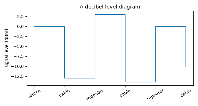
A 1 mW source feeds a chain of cable sections (loss) and repeaters (gain).

stages = [("cable", 0.05), ("repeater", 40.0), ("cable", 0.02), ("repeater", 25.0), ("cable", 0.1)]
linear = 1e-3 * np.prod([g for _, g in stages])
in_db = float(dbm(1e-3)) + sum(float(db(g)) for _, g in stages)
print(f"linear product: {linear:.4e} W, decibel sum: {in_db:.2f} dBm -> {float(from_dbm(in_db)):.4e} W")
assert np.isclose(from_dbm(in_db), linear)

linear product: 1.0000e-04 W, decibel sum: -10.00 dBm -> 1.0000e-04 W

Reference points worth memorising

for ratio in [2, 10, 100, 0.5]:
    print(f"x{ratio:<5} = {float(db(ratio)):+6.2f} dB")
assert np.isclose(from_db(3.0103), 2, rtol=1e-4)

level = [float(dbm(1e-3))]
for _, g in stages:
    level.append(level[-1] + float(db(g)))
fig, ax = plt.subplots(figsize=(6.5, 3.5))
ax.step(range(len(level)), level, where="post")
ax.set_xticks(range(len(level)), ["source"] + [name for name, _ in stages], rotation=30)
ax.set(ylabel="signal level [dBm]", title="A decibel level diagram")
fig.tight_layout()

plt.show()

x2     =  +3.01 dB
x10    = +10.00 dB
x100   = +20.00 dB
x0.5   =  -3.01 dB