Fessenden’s amplitude modulation

On Christmas Eve 1906 Reginald Fessenden is said to have broadcast voice and music from Brant Rock, Massachusetts, by varying the amplitude of a continuous high-frequency wave. Conventional AM, \(s(t) = A_c[1+\mu m(t)]\cos 2\pi f_c t\) (am_signal()), keeps the carrier so a simple envelope detector can recover the message, provided the modulation index stays at or below one. The spectrum shows the cost: a strong carrier and two sidebands, so at most one third of the power carries the message.

import matplotlib.pyplot as plt
import numpy as np
from scipy.signal import hilbert

from engineeringkit.communications import am_signal

Envelope detection works only without overmodulation

fs, fc, fm = 200e3, 10e3, 500.0
t = np.arange(0, 0.01, 1 / fs)
freq = np.fft.rfftfreq(t.size, 1 / fs)
message = np.cos(2 * np.pi * fm * t)
fig, axes = plt.subplots(2, 2, figsize=(10, 5.5))
for col, mu in enumerate([0.7, 1.5]):
    s = am_signal(message, t, fc, mu=mu)
    envelope = np.abs(hilbert(s))
    error = np.max(np.abs(envelope[200:-200] - 1 - mu * message[200:-200]))
    print(f"mu = {mu}: max envelope-detector error = {error:.3f}")
    axes[0, col].plot(t * 1e3, s, lw=0.5)
    axes[0, col].plot(t * 1e3, envelope, "C3")
    axes[0, col].set(title=f"modulation index {mu}", xlabel="time [ms]")
    axes[1, col].stem(freq / 1e3, np.abs(np.fft.rfft(s)) / t.size, markerfmt=" ", basefmt=" ")
    axes[1, col].set(xlim=(8, 12), xlabel="frequency [kHz]")
fig.tight_layout()

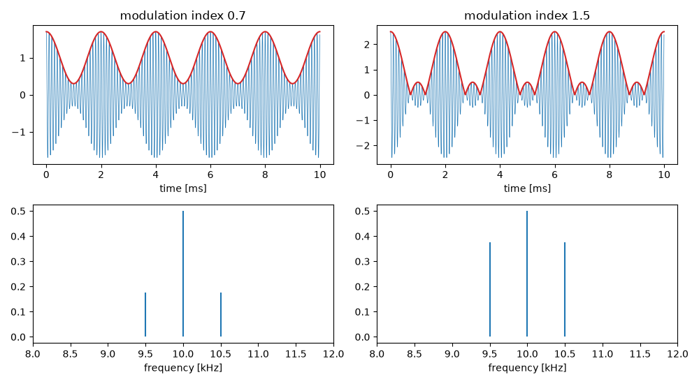
mu = 0.7: max envelope-detector error = 0.000
mu = 1.5: max envelope-detector error = 1.000

Carrier and sidebands

For a tone, sideband power is \(\mu^2/(2+\mu^2)\) of the total, at most one third.

mu = 1.0
power = np.abs(np.fft.rfft(am_signal(message, t, fc, mu=mu))) ** 2
carrier = power[np.argmin(np.abs(freq - fc))]
efficiency = 1 - carrier / power.sum()
print(f"mu = 1: sideband share of power = {efficiency:.3f} (theory 1/3)")
assert np.isclose(efficiency, mu**2 / (2 + mu**2), atol=1e-3)

plt.show()

mu = 1: sideband share of power = 0.333 (theory 1/3)