Johnson-Nyquist thermal noise

In 1926-1928 John B. Johnson at Bell Labs measured a random voltage across every resistor, proportional to its resistance and absolute temperature and independent of its material. Harry Nyquist explained it from thermodynamics: the available noise power in a bandwidth \(B\) is \(kTB\) (thermal_noise_power()), -174 dBm/Hz at 290 K. This example synthesises white Gaussian noise with that power, measures it after band-limiting, and recovers the open-circuit voltage \(\sqrt{4kTRB}\).

import matplotlib.pyplot as plt
import numpy as np

from engineeringkit.communications import BOLTZMANN, dbm, thermal_noise_power

-174 dBm per hertz

print(f"kT at 290 K: {float(dbm(thermal_noise_power(1.0))):.2f} dBm/Hz")
print(f"noise in a 6 MHz TV channel: {float(dbm(thermal_noise_power(6e6))):.1f} dBm")

kT at 290 K: -173.98 dBm/Hz
noise in a 6 MHz TV channel: -106.2 dBm

Simulated resistor noise

A 50 ohm resistor at 300 K sampled at 1 GHz: the open-circuit RMS voltage in the full 500 MHz Nyquist band is \(\sqrt{4kTRB}\), and the power delivered to a matched load is \(kTB\).

rng = np.random.default_rng(1928)
R, T, fs = 50.0, 300.0, 1e9
B = fs / 2
v_rms = np.sqrt(4 * BOLTZMANN * T * R * B)
v = rng.normal(0, v_rms, 2**18)
matched_power = np.mean((v / 2) ** 2) / R
print(f"v_rms = {v_rms * 1e6:.2f} uV; matched-load power {matched_power:.3e} W vs kTB {float(thermal_noise_power(B, T)):.3e} W")
assert np.isclose(matched_power, thermal_noise_power(B, T), rtol=0.02)

spectrum = np.abs(np.fft.rfft(v)) ** 2 / (fs * v.size) * 2
freq = np.fft.rfftfreq(v.size, 1 / fs)
fig, axes = plt.subplots(1, 2, figsize=(10, 3.5))
axes[0].plot(np.arange(400) / fs * 1e9, v[:400] * 1e6, lw=0.7)
axes[0].set(xlabel="time [ns]", ylabel="voltage [uV]", title="Johnson noise, 50 ohm at 300 K")
axes[1].semilogy(freq[1::64] / 1e6, spectrum[1::64], ".", ms=2)
axes[1].axhline(4 * BOLTZMANN * T * R, color="C3", label="4kTR (flat)")
axes[1].set(xlabel="frequency [MHz]", ylabel="voltage PSD [V²/Hz]")
axes[1].legend()
fig.tight_layout()

plt.show()

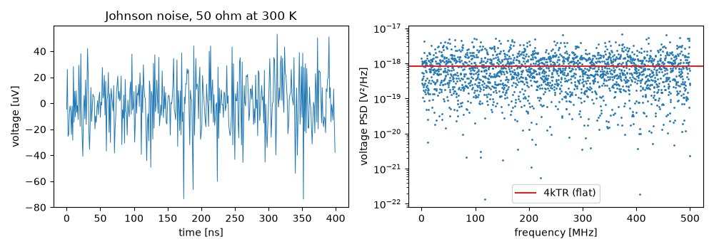
v_rms = 20.35 uV; matched-load power 2.069e-12 W vs kTB 2.071e-12 W