Kochenburger’s describing function (1950)

Ralph Kochenburger, working on relay-driven propeller pitch controls, replaced a nonlinearity by the gain \(N(A)\) it offers to the fundamental of a sinusoid of amplitude \(A\) (relay_describing_function(), saturation_describing_function()). A loop \(L(s)\) closed through it can then oscillate where \(L(j\omega) = -1/N(A)\): at a phase crossover, with \(N(A)\) equal to the gain margin (limit_cycle()). For an ideal relay \(N = 4M/(\pi A)\) and \(L = 1/(s+1)^3\), the cycle is at \(\omega = \sqrt3\) with \(A = M/(2\pi)\). This is also the relay experiment that autotuners use to find Ziegler and Nichols’s ultimate point. The method is approximate because the loop does not filter out the harmonics completely, so each prediction is checked against a simulation of the nonlinear loop.

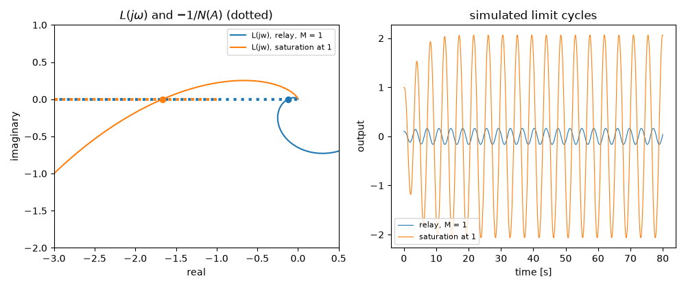
relay, M = 1: predicted A = 0.1592, T = 3.628 s; simulated A = 0.1631, T = 3.680 s; stable: True
saturation at 1: predicted A = 2.0331, T = 4.443 s; simulated A = 2.0652, T = 4.489 s; stable: True

import matplotlib.pyplot as plt
import numpy as np
from scipy import signal

from engineeringkit.control_systems import (
    limit_cycle,
    nyquist,
    relay_describing_function,
    saturation_describing_function,
    transfer_function,
)
from engineeringkit.integrators import integrate_ode


def simulate(loop, nonlinearity, t, start=40.0):
    """Close ``loop`` through ``nonlinearity`` of the error; return y and the late amplitude and period."""
    A, B, C, _ = signal.tf2ss(loop.num, loop.den)
    sol = integrate_ode(lambda _, x: A @ x + B.ravel() * nonlinearity(-(C.ravel() @ x)), np.r_[np.zeros(len(A) - 1), 0.1], t, "rk4")
    y = sol.history @ C.ravel()
    late = t > start
    rising = np.flatnonzero((y[:-1] < 0) & (y[1:] >= 0))
    return y, np.ptp(y[late]) / 2, np.mean(np.diff(t[rising[t[rising] > start]]))


fig, axs = plt.subplots(1, 2, figsize=(10, 4.2))
cases = [
    ("relay, M = 1", transfer_function([1], [1, 3, 3, 1]), np.sign, lambda A: relay_describing_function(A, 1.0)),
    (
        "saturation at 1",
        transfer_function([10], [1, 3, 2, 0]),
        lambda e: np.clip(e, -1, 1),
        lambda A: saturation_describing_function(A, 1.0),
    ),
]
t = np.linspace(0, 80, 80001)
for label, loop, nonlinearity, describing in cases:
    (cycle,) = limit_cycle(loop, describing, (0.01, 100))
    y, amplitude, period = simulate(loop, nonlinearity, t)
    print(
        f"{label}: predicted A = {cycle['amplitude']:.4f}, T = {cycle['period']:.3f} s; "
        f"simulated A = {amplitude:.4f}, T = {period:.3f} s; stable: {cycle['stable']}"
    )
    assert cycle["stable"] and abs(amplitude / cycle["amplitude"] - 1) < 0.04 and abs(period / cycle["period"] - 1) < 0.02
    axs[1].plot(t, y, lw=0.8, label=label)

    # -1/N(A) on the Nyquist plane meets L(jw) at the predicted cycle.
    w = np.logspace(-1, 1, 2000)
    h = nyquist(loop, w)
    (line,) = axs[0].plot(h.real, h.imag, label=f"L(jw), {label}")
    amplitudes = np.logspace(-2, 2, 400)
    critical = -1 / np.asarray(describing(amplitudes), float)
    axs[0].plot(critical, 0 * critical, ":", lw=3, color=line.get_color())
    axs[0].plot(-1 / describing(cycle["amplitude"]), 0, "o", color=line.get_color())

axs[0].set(xlim=(-3, 0.5), ylim=(-2, 1), xlabel="real", ylabel="imaginary", title=r"$L(j\omega)$ and $-1/N(A)$ (dotted)")
axs[0].legend(fontsize=8)
axs[1].set(xlabel="time [s]", ylabel="output", title="simulated limit cycles")
axs[1].legend(fontsize=8)
fig.tight_layout()
plt.show()