Kalman’s linear-quadratic regulator (1960)

Rudolf Kalman (1960) asked for the state feedback \(u = -Kx\) that minimises \(J = \int_0^\infty (x^\mathsf{T}Qx + u^\mathsf{T}Ru)\,dt\). The answer is \(K = R^{-1}B^\mathsf{T}P\), where \(P\) solves an algebraic Riccati equation, and the minimum cost from \(x_0\) is \(x_0^\mathsf{T}Px_0\) (lqr()). The weights replace pole locations as the designer’s knobs: a cheaper input (smaller \(R\)) buys a faster response.

For the double integrator \(\ddot y = u\) with \(Q = \mathrm{diag}(1, 0)\) and \(R = r\), the gain is \(K = [r^{-1/2},\ \sqrt2\,r^{-1/4}]\): a closed-loop damping ratio of \(1/\sqrt2\) for every \(r\).

import matplotlib.pyplot as plt
import numpy as np
from scipy.integrate import solve_ivp

from engineeringkit.control_systems import discretize_zoh, dlqr, lqr

A = np.array([[0.0, 1.0], [0.0, 0.0]])
B = np.array([[0.0], [1.0]])
Q = np.diag([1.0, 0.0])
x0 = np.array([1.0, 0.0])

fig, (ax1, ax2) = plt.subplots(2, 1, sharex=True, figsize=(7, 6))
for r in (0.01, 0.1, 1.0):
    K, P, closed = lqr(A, B, Q, [[r]])
    assert np.allclose(K, [[r**-0.5, np.sqrt(2) * r**-0.25]])
    zeta = -closed.real[0] / np.abs(closed[0])
    assert np.isclose(zeta, 1 / np.sqrt(2))

    # Simulate the closed loop, integrating the cost alongside the state.
    def rhs(t, z, K=K, r=r):
        x = z[:2]
        u = -(K @ x)
        return np.concatenate((A @ x + B @ u, [x @ Q @ x + r * u[0] ** 2]))

    sol = solve_ivp(rhs, (0, 40), np.concatenate((x0, [0.0])), rtol=1e-10, atol=1e-12, dense_output=True)
    cost = sol.y[2, -1]
    print(f"r = {r:5.2f}: K = {K.round(3).tolist()}, J = {cost:.5f}, x0'Px0 = {x0 @ P @ x0:.5f}")
    assert np.isclose(cost, x0 @ P @ x0, rtol=1e-6)

    t = np.linspace(0, 8, 400)
    x = sol.sol(t)[:2]
    ax1.plot(t, x[0], label=f"r = {r}")
    ax2.plot(t, -(K @ x)[0], label=f"r = {r}")

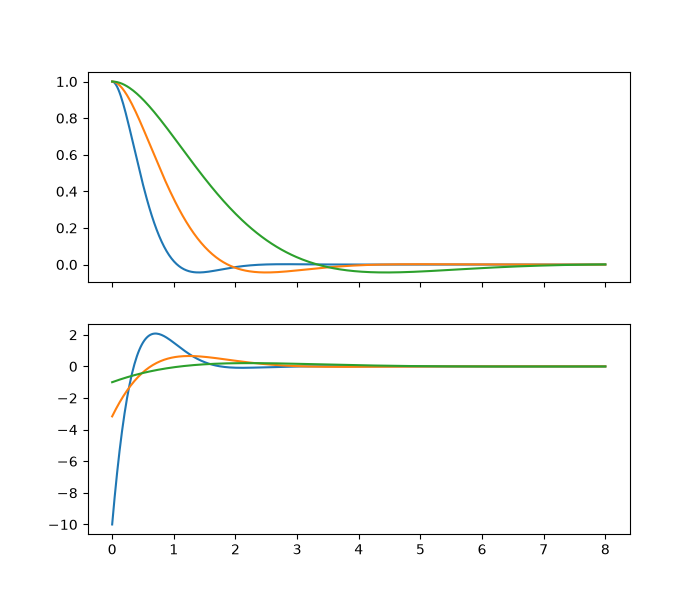
r =  0.01: K = [[10.0, 4.472]], J = 0.44721, x0'Px0 = 0.44721
r =  0.10: K = [[3.162, 2.515]], J = 0.79527, x0'Px0 = 0.79527
r =  1.00: K = [[1.0, 1.414]], J = 1.41421, x0'Px0 = 1.41421

The discrete regulator converges to the continuous one

Bellman’s dynamic programming over sampling periods gives the discrete Riccati equation (dlqr()). With the weights scaled by the period, its gain tends to the continuous gain as the period shrinks.

K, _, _ = lqr(A, B, Q, [[0.1]])
for dt in (0.1, 0.01, 0.001):
    Ad, Bd = discretize_zoh(A, B, dt)
    Kd, _, _ = dlqr(Ad, Bd, Q * dt, [[0.1 * dt]])
    print(f"dt = {dt}: discrete gain {Kd.round(4).tolist()}")
assert np.allclose(Kd, K, rtol=2e-3)

ax1.set(ylabel="position y", title="LQR from y(0) = 1")
ax2.set(xlabel="time [s]", ylabel="input u")
ax1.legend()

plt.show()

dt = 0.1: discrete gain [[2.7889, 2.3617]]
dt = 0.01: discrete gain [[3.1228, 2.4991]]
dt = 0.001: discrete gain [[3.1583, 2.5133]]