Evans’s root locus

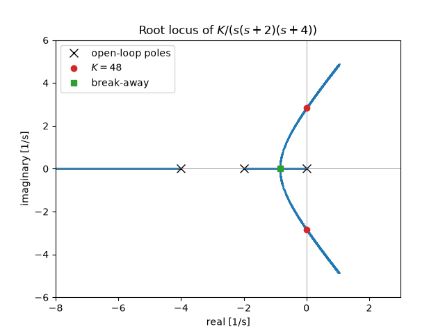
Walter Evans at North American Aviation (1948) showed how to sketch the paths of the closed-loop poles as a single gain \(K\) rises from zero, without solving a polynomial for each gain (root_locus()). For \(K/(s(s+2)(s+4))\) the branches leave the poles at 0, -2 and -4. Two of them meet and break away from the real axis where \(\tfrac{d}{ds}[s(s+2)(s+4)] = 0\), at \(s = -2 + 2/\sqrt3\). They cross the imaginary axis at \(\pm j\sqrt8\) when \(K = 48\).

import matplotlib.pyplot as plt
import numpy as np

from engineeringkit.control_systems import root_locus
from engineeringkit.control_systems.visualizers import plot_root_locus

num, den = [1.0], [1.0, 6.0, 8.0, 0.0]

Break-away point and imaginary-axis crossing

s_b = -2 + 2 / np.sqrt(3)
K_b = -np.polyval(den, s_b)
pair = np.sort_complex(root_locus(num, den, [K_b])[0])[1:]
print(f"break-away at s = {s_b:.4f} for K = {K_b:.4f}: roots {np.round(pair, 3)}")
assert np.allclose(pair, s_b, atol=1e-4)

crossing = root_locus(num, den, [48.0])[0]
print("K = 48 roots:", np.round(crossing, 6))
assert np.isclose(np.abs(crossing.imag).max(), np.sqrt(8)) and abs(crossing.real[np.argmax(crossing.imag)]) < 1e-9

ax = plot_root_locus(num, den, np.concatenate((np.linspace(0, 5, 400), np.linspace(5, 200, 800))))
ax.plot([0, 0], [-np.sqrt(8), np.sqrt(8)], "C3o", label="$K = 48$")
ax.plot(s_b, 0, "C2s", label="break-away")
ax.set(xlim=(-8, 3), ylim=(-6, 6), title=r"Root locus of $K/(s(s+2)(s+4))$")
ax.legend()

plt.show()

break-away at s = -0.8453 for K = 3.0792: roots [-0.845+0.j -0.845+0.j]
K = 48 roots: [-6.+0.j        0.+2.828427j  0.-2.828427j]