Tustin’s bilinear transform (1947)

Arnold Tustin, analysing servomechanisms at Metropolitan-Vickers, turned continuous dynamics into recurrences on sampled values by substituting \(s \to (2/T)(z - 1)/(z + 1)\), which integrates by the trapezoidal rule (discretize_tustin()). The whole left half-plane maps into the unit disc, so a stable model stays stable, but the frequency axis is compressed: a continuous frequency \(\omega\) appears at \((2/T)\arctan(\omega T/2)\). A sharp resonance near the Nyquist frequency moves. Prewarping, substituting \(\omega_0/\tan(\omega_0T/2)\) for \(2/T\), puts it back exactly at \(\omega_0\).

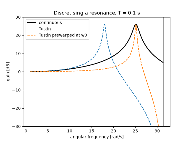
Tustin: resonance at 17.967 rad/s (continuous 25.133)
Tustin prewarped at w0: resonance at 25.129 rad/s (continuous 25.133)

import matplotlib.pyplot as plt
import numpy as np

from engineeringkit.control_systems import discretize_tustin, nyquist, poles, transfer_function

T = 0.1
w0 = 0.8 * np.pi / T  # a resonance at 80% of the Nyquist frequency
G = transfer_function([w0**2], [1, 0.05 * w0, w0**2])
w = np.linspace(1, np.pi / T, 200001)
z = np.exp(1j * w * T)

fig, ax = plt.subplots()
ax.plot(w, 20 * np.log10(np.abs(nyquist(G, w))), "k", lw=2, label="continuous")
for label, prewarp in (("Tustin", None), ("Tustin prewarped at w0", w0)):
    Gd = discretize_tustin(G, T, prewarp_frequency=prewarp)
    assert np.all(np.abs(np.roots(Gd.den)) < 1)
    response = np.polyval(Gd.num, z) / np.polyval(Gd.den, z)
    peak = w[np.argmax(np.abs(response))]
    print(f"{label}: resonance at {peak:.3f} rad/s (continuous {w0:.3f})")
    ax.plot(w, 20 * np.log10(np.abs(response)), "--", label=label)
    if prewarp is None:
        # The trapezoidal map moves the peak to (2/T) arctan(w0 T / 2).
        assert abs(peak - 2 / T * np.arctan(w0 * T / 2)) < 0.02
        c = 2 / T
        expected = (c + poles(G)) / (c - poles(G))
        assert np.allclose(np.sort_complex(np.roots(Gd.den)), np.sort_complex(expected))
    else:
        assert abs(peak - w0) < 0.01
        assert np.isclose(np.polyval(Gd.num, np.exp(1j * w0 * T)) / np.polyval(Gd.den, np.exp(1j * w0 * T)), nyquist(G, w0))
ax.axvline(np.pi / T, color="gray", lw=0.6)
ax.set(xlabel="angular frequency [rad/s]", ylabel="gain [dB]", ylim=(-30, 30), title=f"Discretising a resonance, T = {T} s")
ax.legend()
plt.show()