Hurwitz’s determinant test

Aurel Stodola, designing turbine regulators in Zürich, asked Adolf Hurwitz for a practical stability condition. Hurwitz (1895), unaware of Routh’s work, gave it as determinants: build the matrix \(H_{ij} = a_{2j-i}\) from the coefficients, and every root lies in the left half-plane exactly when all leading minors are positive (hurwitz_determinants()). At the boundary \(\Delta_{n-1}\) passes through zero as a pair of roots crosses the imaginary axis.

import matplotlib.pyplot as plt
import numpy as np

from engineeringkit.control_systems import hurwitz_determinants

A quartic family

The roots of \((s+1)^4 + K\) are \(-1 + K^{1/4}e^{i(\pi/4 + k\pi/2)}\), so the rightmost pair reaches the imaginary axis at \(K = 4\).

gains = np.linspace(0.1, 8, 400)
deltas = np.array([hurwitz_determinants(np.poly([-1, -1, -1, -1]) + [0, 0, 0, 0, K]) for K in gains])
rightmost = np.array([np.roots(np.poly([-1, -1, -1, -1]) + [0, 0, 0, 0, K]).real.max() for K in gains])
stable_by_hurwitz = np.all(deltas > 0, axis=1)
assert np.array_equal(stable_by_hurwitz, rightmost < 0)
boundary = gains[np.argmin(np.abs(deltas[:, 2]))]
print(f"Delta_3 vanishes near K = {boundary:.3f} (exact 4)")
assert abs(boundary - 4) < 0.02

fig, axes = plt.subplots(1, 2, figsize=(10, 3.8))
for k in range(4):
    axes[0].plot(gains, deltas[:, k], label=rf"$\Delta_{k + 1}$")
axes[0].axhline(0, color="k", lw=0.8)
axes[0].axvline(4, color="C3", ls="--", lw=0.8)
axes[0].set(xlabel="$K$", ylabel="Hurwitz minor", ylim=(-60, 120))
axes[0].legend()
axes[1].plot(gains, rightmost)
axes[1].axhline(0, color="k", lw=0.8)
axes[1].set(xlabel="$K$", ylabel="largest real part of a root")
fig.tight_layout()

plt.show()

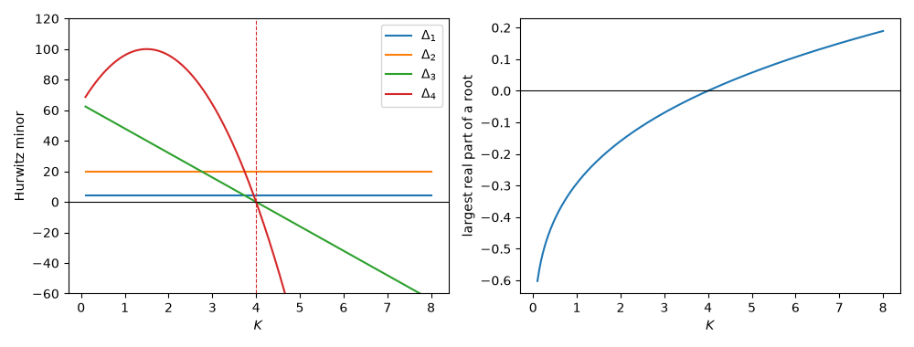
Delta_3 vanishes near K = 4.001 (exact 4)