Steinmetz’s phasors and complex impedance (1893)

AC circuits obey linear differential equations, and before 1893 engineers solved them with trigonometry and graphical constructions. At the International Electrical Congress in Chicago, Charles Proteus Steinmetz showed that a sinusoid \(A\cos(\omega t + \phi)\) can be carried as the complex number \(Ae^{j\phi}\). Differentiation becomes multiplication by \(j\omega\), so an inductor becomes the impedance \(j\omega L\) (inductor_impedance()), a capacitor \(1/j\omega C\) (capacitor_impedance()), and AC circuits are solved by Ohm’s law with complex numbers (series_rlc_impedance()). This example solves a series RLC circuit by phasors and checks the answer against a time-domain simulation.

import matplotlib.pyplot as plt
import numpy as np
from scipy.integrate import solve_ivp

from engineeringkit.electrical_engineering import (
    capacitor_impedance,
    inductor_impedance,
    phasor,
    polar,
    series_rlc_impedance,
)
from engineeringkit.electrical_engineering.visualizers import plot_phasors

Phasor solution

R, L, C, f, Vm = 30.0, 0.1, 50e-6, 50.0, 100.0
w = 2 * np.pi * f
Z = series_rlc_impedance(R, L, C, w)
I = phasor(Vm, 0.0) / Z
magnitude, phase = polar(I)
print(f"Z = {Z:.2f} ohm, I = {magnitude:.3f} A at {np.degrees(phase):.1f} degrees")
VR, VL, VC = I * R, I * inductor_impedance(L, w), I * capacitor_impedance(C, w)
assert np.isclose(VR + VL + VC, Vm)  # Kirchhoff's voltage law holds for phasors

Z = 30.00-32.25j ohm, I = 2.270 A at 47.1 degrees

Time-domain check

Integrate \(L\,di/dt + Ri + q/C = V_m\cos\omega t\) for 40 cycles and compare the steady state with \(|I|\cos(\omega t + \arg I)\).

def rhs(t, x):
    q, i = x
    return [i, (Vm * np.cos(w * t) - R * i - q / C) / L]


t_end = 40 / f
sol = solve_ivp(rhs, (0, t_end), [0, 0], rtol=1e-9, atol=1e-12, dense_output=True)
t = np.linspace(t_end - 2 / f, t_end, 400)
i_sim = sol.sol(t)[1]
i_phasor = magnitude * np.cos(w * t + phase)
print(f"largest difference after 40 cycles: {np.max(np.abs(i_sim - i_phasor)):.1e} A")
assert np.allclose(i_sim, i_phasor, atol=1e-4 * magnitude)

fig, axes = plt.subplots(1, 2, figsize=(10, 4))
plot_phasors([Vm, VR, VL, VC, I * 50], labels=["$V$", "$V_R$", "$V_L$", "$V_C$", "$I$ (x50)"], ax=axes[0])
axes[0].set_title("Phasor diagram")
axes[1].plot(t * 1e3, i_sim, label="ODE simulation")
axes[1].plot(t * 1e3, i_phasor, "--", label="phasor solution")
axes[1].set(xlabel="time [ms]", ylabel="current [A]", title="Steady state")
axes[1].legend()
fig.tight_layout()

plt.show()

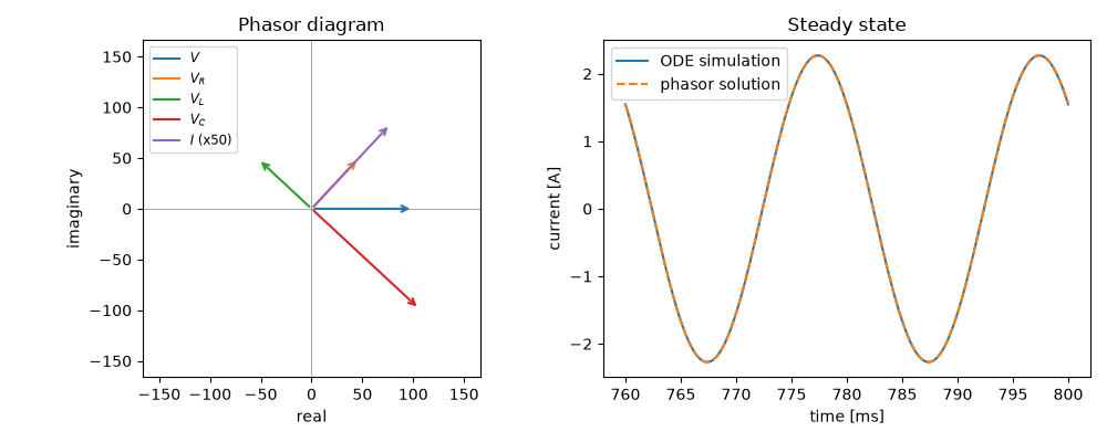
largest difference after 40 cycles: 1.4e-09 A