Ohm’s law (1827)

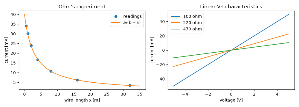
In 1826 Georg Simon Ohm drove current from a thermocouple, a steady source, through brass wires of different lengths \(x\) and read the current on a torsion galvanometer. The readings fitted \(X = a/(b + x)\): a fixed “exciting force” \(a\) divided by the total resistance of the wire plus the rest of the circuit, \(b\). In modern form that is \(V = IR\) (ohms_law()). This example rebuilds Ohm’s experiment, recovers the source voltage and internal resistance from the readings, and checks the series and parallel rules that follow from the law.

import matplotlib.pyplot as plt
import numpy as np

from engineeringkit.electrical_engineering import ohms_law, parallel_resistance, series_resistance

Ohm’s wires

A thermocouple of EMF 2 mV and internal resistance 0.05 ohm drives copper wire of 0.017 ohm per metre. The current falls as the wire lengthens, exactly as \(a/(b + x)\), with measurement noise of 1%.

rng = np.random.default_rng(1827)
emf, r_internal, r_per_m = 2e-3, 0.05, 0.017
lengths = np.array([0.5, 1, 2, 4, 8, 16, 32])
total = np.array([series_resistance(r_internal, r_per_m * x) for x in lengths])
current = np.array([ohms_law(voltage=emf, resistance=R) for R in total]) * (1 + 0.01 * rng.standard_normal(lengths.size))

# 1/I is linear in x: 1/I = (r_internal + r_per_m x) / emf.
slope, intercept = np.polyfit(lengths, 1 / current, 1)
emf_fit = r_per_m / slope
r_fit = intercept * emf_fit
print(f"fitted EMF {emf_fit * 1e3:.3f} mV (true 2.000), internal resistance {r_fit:.4f} ohm (true 0.0500)")

fitted EMF 2.026 mV (true 2.000), internal resistance 0.0515 ohm (true 0.0500)

Series and parallel

Equal current through resistors in series means their voltages add, so resistances add. Equal voltage across resistors in parallel means their currents add, so conductances add.

R = [100.0, 220.0, 470.0]
V = 10.0
i_series = ohms_law(voltage=V, resistance=series_resistance(*R))
assert np.isclose(sum(i_series * r for r in R), V)
i_parallel = sum(ohms_law(voltage=V, resistance=r) for r in R)
assert np.isclose(i_parallel, ohms_law(voltage=V, resistance=parallel_resistance(*R)))
print(f"series {series_resistance(*R):.0f} ohm, parallel {parallel_resistance(*R):.2f} ohm")

fig, axes = plt.subplots(1, 2, figsize=(10, 3.6))
x = np.linspace(0, 35, 200)
axes[0].plot(lengths, current * 1e3, "o", label="readings")
axes[0].plot(x, emf / (r_internal + r_per_m * x) * 1e3, label="$a/(b + x)$")
axes[0].set(xlabel="wire length x [m]", ylabel="current [mA]", title="Ohm's experiment")
axes[0].legend()
v = np.linspace(-5, 5, 11)
for r in R:
    axes[1].plot(v, [ohms_law(voltage=vk, resistance=r) * 1e3 for vk in v], label=f"{r:.0f} ohm")
axes[1].set(xlabel="voltage [V]", ylabel="current [mA]", title="Linear V-I characteristics")
axes[1].legend()
fig.tight_layout()

assert abs(emf_fit - emf) / emf < 0.03 and abs(r_fit - r_internal) / r_internal < 0.1

plt.show()

series 790 ohm, parallel 59.98 ohm