Jacobi’s maximum power theorem (c. 1840)

Around 1840 Moritz von Jacobi, building battery-powered electric motors in St Petersburg (one drove a boat on the Neva), asked what load draws the most power from a battery. A source of EMF \(V\) and internal resistance \(R_s\) delivers \(P = V^2 R_L/(R_s + R_L)^2\) to a load \(R_L\), largest when \(R_L = R_s\) (maximum_power_transfer()). At that match the source wastes as much as it delivers, so the efficiency is only 50%. Engineers later learned to read the theorem the other way: power grids run far from the match, at high efficiency, while radio receivers match to capture every last picowatt.

import matplotlib.pyplot as plt
import numpy as np

from engineeringkit.electrical_engineering import maximum_power_transfer, ohms_law, series_resistance

Sweeping the load

V, Rs = 12.0, 4.0
RL = np.logspace(-1, 2, 601)
I = np.array([ohms_law(voltage=V, resistance=series_resistance(Rs, r)) for r in RL])
P_load = I**2 * RL
efficiency = RL / (Rs + RL)

R_match, P_max = maximum_power_transfer(V, Rs)
best = RL[np.argmax(P_load)]
print(f"numerical optimum R_L = {best:.3f} ohm, theorem {R_match:.1f} ohm; P_max = {P_max:.1f} W")
print(f"efficiency at the match {np.interp(R_match, RL, efficiency):.0%}")
assert np.isclose(best, R_match, rtol=0.01)
assert np.isclose(P_load.max(), P_max, rtol=1e-4)

fig, ax = plt.subplots()
ax.semilogx(RL / Rs, P_load / P_max, label="load power / $P_{max}$")
ax.semilogx(RL / Rs, efficiency, label="efficiency")
ax.axvline(1, color="gray", ls="--")
ax.set(xlabel="$R_L / R_s$", ylabel="fraction", title="Jacobi's maximum power theorem")
ax.legend()

plt.show()

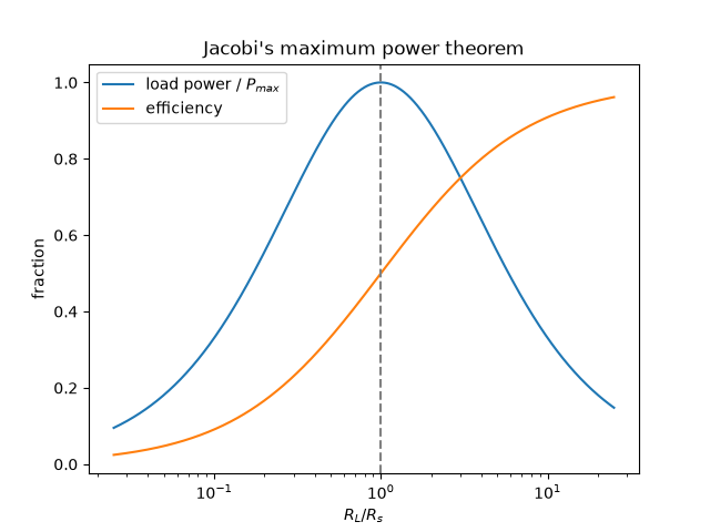
numerical optimum R_L = 3.981 ohm, theorem 4.0 ohm; P_max = 9.0 W
efficiency at the match 50%