Hardy Cross’s method for pipe networks (1936)

A city’s water mains form loops, and the flow in each pipe is fixed by two sets of conditions: continuity at every junction, and zero net head loss round every loop. In 1936 Hardy Cross, at the University of Illinois, proposed solving them by hand: guess flows that satisfy continuity, then correct one loop at a time by \(\Delta Q = -\sum r Q|Q|/(2\sum r|Q|)\), a Newton step that leaves the junctions balanced (hardy_cross()). It was the standard method until computers took over. This example balances a two-loop network sized with Darcy-Weisbach resistances (pipe_resistance()).

import matplotlib.pyplot as plt
import numpy as np
from scipy import optimize

from engineeringkit.fluid_engineering import hardy_cross, pipe_resistance

The network

Water enters at junction A (100 L/s) and leaves at B (30 L/s), C (40 L/s) and D (30 L/s). Five pipes, each with a reference direction: A→B, B→D, A→C, C→D and B→C. Loop I is A-B-C, loop II is B-D-C; clockwise counts as positive.

lengths = np.array([300.0, 400.0, 400.0, 300.0, 300.0])
diameters = np.array([0.30, 0.20, 0.25, 0.20, 0.15])
r = pipe_resistance(0.02, lengths, diameters)
loops = np.array([[1, 0, -1, 0, 1], [0, 1, 0, -1, -1]])
Q0 = np.array([0.060, 0.030, 0.040, 0.000, 0.000])  # satisfies continuity

result = hardy_cross(r, loops, Q0)
for name, q, h in zip(["A-B", "B-D", "A-C", "C-D", "B-C"], result.flows, result.head_losses):
    print(f"pipe {name}: {1e3 * q:6.2f} L/s, head loss {h:5.2f} m")
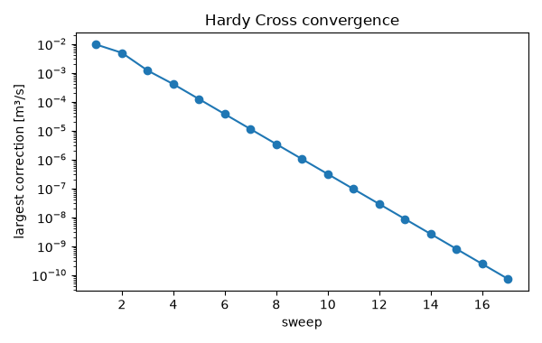
print(result.summary()["iterations"], "sweeps")

fig, ax = result.plot()
fig.set_size_inches(6, 3.8)
fig.tight_layout()

pipe A-B:  57.74 L/s, head loss  0.68 m
pipe B-D:  18.74 L/s, head loss  0.73 m
pipe A-C:  42.26 L/s, head loss  1.21 m
pipe C-D:  11.26 L/s, head loss  0.20 m
pipe B-C:   9.00 L/s, head loss  0.53 m
17 sweeps

Checking against a direct solve

Junction continuity (three independent equations) and the two loop equations, solved together by Newton’s method, give the same flows.

incidence = np.array([[-1, 0, -1, 0, 0], [1, -1, 0, 0, -1], [0, 0, 1, -1, 1], [0, 1, 0, 1, 0]])
demand = incidence @ Q0


def equations(q):
    return np.concatenate([(incidence @ q - demand)[:3], loops @ (r * q * np.abs(q))])


direct = optimize.fsolve(equations, Q0, xtol=1e-13)
print(f"largest difference from the direct solve: {np.abs(direct - result.flows).max():.1e} m³/s")

assert np.allclose(incidence @ result.flows, demand)
assert np.abs(result.loop_residuals).max() < 1e-6
assert np.allclose(result.flows, direct, atol=1e-9)

plt.show()

largest difference from the direct solve: 3.2e-11 m³/s