Joukowsky’s water hammer (1898)

Burst mains in Moscow’s new water system led Nikolai Joukowsky to a series of experiments in 1897, with pipes up to 760 m long. He reported in 1898 that closing a valve suddenly raises the pressure by \(\Delta p = \rho a \Delta v\) (water_hammer_pressure()), where \(a\) is the speed of the pressure wave, slowed below the speed of sound in water by the elasticity of the pipe wall (Korteweg’s formula, pipe_wave_speed()). The wave runs to the reservoir and back in \(2L/a\) (critical_closure_time()), and a valve closed faster than that sees the full rise. This example compares pipe materials and draws the pressure at the valve.

import matplotlib.pyplot as plt
import numpy as np

from engineeringkit.fluid_engineering import (
    critical_closure_time,
    hydrostatic_pressure,
    pipe_wave_speed,
    water_hammer_pressure,
)

Wave speed and surge by pipe material

Water (\(K = 2.2\) GPa) at 2 m/s in a 300 mm pipe.

K, rho, D, v0 = 2.2e9, 998.0, 0.3, 2.0
materials = {"steel": (200e9, 0.008), "ductile iron": (170e9, 0.010), "PVC": (3.0e9, 0.015), "rigid": (np.inf, 1.0)}
for name, (E, e) in materials.items():
    a = np.sqrt(K / rho) if np.isinf(E) else pipe_wave_speed(K, rho, D, e, E)
    print(f"{name:>12}: a = {a:6.0f} m/s, surge {water_hammer_pressure(rho, a, v0) / 1e6:.2f} MPa")

       steel: a =   1249 m/s, surge 2.49 MPa
ductile iron: a =   1260 m/s, surge 2.52 MPa
         PVC: a =    375 m/s, surge 0.75 MPa
       rigid: a =   1485 m/s, surge 2.96 MPa

Pressure at the valve

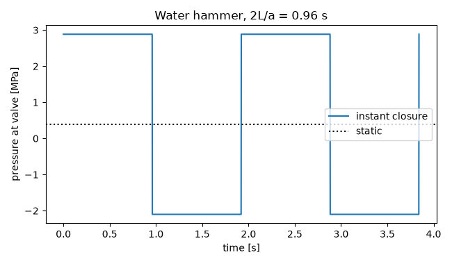
A 600 m steel line from a reservoir with 40 m of head. After an instant closure, and without friction, the valve pressure alternates between the static value plus and minus the surge, with period \(4L/a\). Closing over a time \(T_c\) longer than \(2L/a\) lets the reflected wave arrive first; Michaud’s estimate of the rise is then \(2\rho L v_0/T_c\).

L, H = 600.0, 40.0
a = pipe_wave_speed(K, rho, D, 0.008, 200e9)
dp = water_hammer_pressure(rho, a, v0)
T2 = critical_closure_time(L, a)
t = np.linspace(0, 4 * T2, 2000)
p_static = hydrostatic_pressure(rho, H)
p_valve = p_static + dp * np.where((t % (2 * T2)) < T2, 1.0, -1.0)

fig, ax = plt.subplots(figsize=(6.5, 3.8))
ax.plot(t, p_valve / 1e6, label="instant closure")
ax.axhline(p_static / 1e6, color="k", ls=":", label="static")
ax.set(xlabel="time [s]", ylabel="pressure at valve [MPa]", title=f"Water hammer, 2L/a = {T2:.2f} s")
ax.legend()
fig.tight_layout()

for Tc in [2 * T2, 5 * T2, 10 * T2]:
    print(f"closing in {Tc:.1f} s: rise about {2 * rho * L * v0 / Tc / 1e6:.2f} MPa (Michaud)")

closing in 1.9 s: rise about 1.25 MPa (Michaud)
closing in 4.8 s: rise about 0.50 MPa (Michaud)
closing in 9.6 s: rise about 0.25 MPa (Michaud)

A sudden stop in steel pipe gives a surge of about 2.5 MPa, six times the static pressure; the slow closures stay below it.

assert np.isclose(dp, rho * a * v0) and 1000 < a < np.sqrt(K / rho)
assert np.isclose(2 * rho * L * v0 / T2, dp)  # Michaud equals Joukowsky at Tc = 2L/a
assert p_valve.min() < 0  # gauge pressure falls below zero: the column can separate

plt.show()