The Braggs’ law of X-ray diffraction (1913)

Laue showed in 1912 that crystals diffract X-rays. William Lawrence Bragg, a research student at Cambridge, read the spots as reflections from planes of atoms: waves reflected by neighbouring planes a distance \(d\) apart reinforce when their path difference is a whole number of wavelengths,

\[n\lambda = 2d\sin\theta\]

(bragg_angle()). With his father’s X-ray spectrometer it turned diffraction into a way of measuring crystals. The example builds the powder pattern of BCC iron and FCC copper (diffraction_peaks()), reads the lattice parameter back from a peak, and checks the density it implies.

import matplotlib.pyplot as plt
import numpy as np

from engineeringkit.materials import (
    atomic_packing_factor,
    bragg_angle,
    cubic_lattice_parameter,
    diffraction_peaks,
    interplanar_spacing,
    theoretical_density,
)

One reflection of iron

Iron is BCC with \(a = 0.2866\) nm. With cobalt radiation (\(\lambda = 0.1790\) nm) the (220) planes, \(d = a/\sqrt8\), reflect at \(2\theta \approx 124°\).

a_Fe, wavelength = 0.2866e-9, 0.1790e-9
d220 = interplanar_spacing(a_Fe, 2, 2, 0)
theta = bragg_angle(d220, wavelength)
print(f"d(220) = {d220 * 1e9:.4f} nm, 2 theta = {np.degrees(2 * theta):.2f} deg")
assert np.isclose(wavelength, 2 * d220 * np.sin(theta))

d(220) = 0.1013 nm, 2 theta = 124.08 deg

Powder patterns and the missing peaks

In a BCC cell the atom at the body centre scatters exactly out of phase from the (100) planes, so only planes with \(h + k + l\) even reflect. In FCC the indices must be all odd or all even. The sequence of peaks therefore identifies the structure.

copper_a, Cu_Ka = 0.3615e-9, 0.1542e-9
fe_planes, fe_two_theta = diffraction_peaks(a_Fe, Cu_Ka, "bcc")
cu_planes, cu_two_theta = diffraction_peaks(copper_a, Cu_Ka, "fcc")
for name, planes in (("iron (BCC)", fe_planes), ("copper (FCC)", cu_planes)):
    print(name, ["".join(map(str, p)) for p in planes[:5]])
assert fe_planes[0].tolist() == [1, 1, 0] and cu_planes[0].tolist() == [1, 1, 1]

fig, axs = plt.subplots(2, 1, figsize=(6.5, 4.2), sharex=True)
for ax, planes, angles, name in ((axs[0], fe_planes, fe_two_theta, "iron, BCC"), (axs[1], cu_planes, cu_two_theta, "copper, FCC")):
    ax.vlines(np.degrees(angles), 0, 1)
    for p, t in zip(planes, angles):
        ax.text(np.degrees(t), 1.05, "".join(map(str, p)), ha="center", fontsize=8)
    ax.set(ylim=(0, 1.3), yticks=[], ylabel=name)
axs[1].set_xlabel("2 theta [deg], Cu K-alpha")
fig.tight_layout()

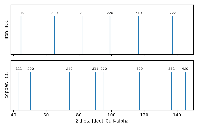
iron (BCC) ['110', '200', '211', '220', '310']
copper (FCC) ['111', '200', '220', '311', '222']

From a peak back to the density

Reading the first copper peak back through Bragg’s law gives the lattice parameter; four atoms of 63.55 g/mol in that cube give the density, and the hard-sphere radius gives the FCC packing factor of 0.74.

d111 = Cu_Ka / (2 * np.sin(cu_two_theta[0] / 2))
a_measured = d111 * np.sqrt(3)
rho = theoretical_density(4, 63.55e-3, a_measured**3)
radius = a_measured / (2 * np.sqrt(2))
print(f"a = {a_measured * 1e9:.4f} nm, R = {radius * 1e9:.4f} nm, density {rho:.0f} kg/m^3, APF {atomic_packing_factor('fcc'):.3f}")
assert np.isclose(cubic_lattice_parameter(radius, "fcc"), copper_a)
assert abs(rho - 8960) / 8960 < 0.01

plt.show()

a = 0.3615 nm, R = 0.1278 nm, density 8935 kg/m^3, APF 0.740