Young’s modulus (1807)

Thomas Young’s Lectures on Natural Philosophy (1807) gave a single number for the stiffness of a material, its “modulus of elasticity”. Young expressed it as the height of a column of the material whose weight would compress it to nothing if the law stayed linear; Navier (1826) restated it as the ratio of stress to strain, \(E = \sigma/\varepsilon\), the form used today (hooke_stress()). The example reduces a simulated tensile test from load and extension to stress and strain (normal_stress(), normal_strain()), fits the modulus with StressStrainCurve and measures the energy the bar absorbs.

import matplotlib.pyplot as plt
import numpy as np

from engineeringkit.materials import StressStrainCurve, hooke_stress, normal_strain, normal_stress, resilience_modulus

From the testing machine to the stress-strain curve

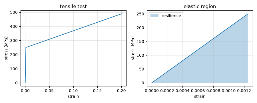
A 10 mm steel bar with a 50 mm gauge length yields at 250 MPa and then hardens linearly. The machine records force and extension; dividing by the original area and length gives engineering stress and strain.

E, sy, H = 200e9, 250e6, 1.2e9
area, gauge = np.pi * 0.005**2, 0.050
strain_in = np.concatenate((np.linspace(0, sy / E, 8), np.linspace(sy / E, 0.20, 200)[1:]))
stress_in = np.where(strain_in <= sy / E, hooke_stress(E, strain_in), sy + H * (strain_in - sy / E))
force, extension = stress_in * area, strain_in * gauge

curve = StressStrainCurve(normal_strain(extension, gauge), normal_stress(force, area))
summary = curve.summary()
print(f"fitted E = {summary['young_modulus_Pa'] / 1e9:.1f} GPa, ultimate {summary['ultimate_strength_Pa'] / 1e6:.0f} MPa")
print(f"toughness {summary['toughness_J_m3'] / 1e6:.1f} MJ/m^3, resilience {resilience_modulus(sy, E) / 1e3:.1f} kJ/m^3")
assert np.isclose(summary["young_modulus_Pa"], E)

fitted E = 200.0 GPa, ultimate 488 MPa
toughness 73.5 MJ/m^3, resilience 156.2 kJ/m^3

Young’s “height of the modulus”

Young’s own measure was a length, \(E/\rho g\). For steel it is thousands of kilometres. The elastic part of the curve stores the modulus of resilience \(\sigma_y^2/2E\), the area of the elastic triangle, which is tiny next to the area under the whole curve.

rho, g = 7850.0, 9.81
print(f"height of the modulus of steel: {E / (rho * g) / 1e3:.0f} km")
elastic = StressStrainCurve(curve.strain[:8], curve.stress[:8])
assert np.isclose(elastic.toughness(), resilience_modulus(sy, E))

fig, (ax1, ax2) = plt.subplots(1, 2, figsize=(9, 3.6))
curve.plot(ax=ax1)
ax1.set_title("tensile test")
elastic.plot(ax=ax2)
ax2.fill_between(elastic.strain, elastic.stress / 1e6, alpha=0.3, label="resilience")
ax2.set_title("elastic region")
ax2.legend()
fig.tight_layout()

plt.show()

height of the modulus of steel: 2597 km