Weibull’s statistical strength of brittle materials (1939)

Identical glass rods or ceramic bars break at widely different loads, and long ones break at lower loads than short ones. Waloddi Weibull, at the Royal Institute of Technology in Stockholm, explained both with a weakest link: a part fails when its worst flaw does, so its survival probability is the product of the survival probabilities of its volume elements,

\[P_f = 1 - \exp\left[-\frac{V}{V_0}\left(\frac{\sigma}{\sigma_0}\right)^m\right]\]

(weibull_failure_probability()). The same distribution later became the standard model of component life, in engineeringkit.reliability.weibull_cdf(), which this function calls. The example fits the Weibull modulus to bend-bar strengths and scales the strength to a larger part (weibull_size_effect()).

import matplotlib.pyplot as plt
import numpy as np

from engineeringkit.materials import weibull_failure_probability, weibull_mean_strength, weibull_size_effect

Fitting a batch of test bars

Thirty alumina bars, each with 10 mm^3 under stress, are drawn from a Weibull population with \(\sigma_0 = 400\) MPa and \(m = 10\). Ranked with Benard’s median rank, \(\ln\ln(1/(1 - P_f))\) against \(\ln\sigma\) is a straight line whose slope is \(m\).

rng = np.random.default_rng(1939)
sigma_0, m_true, V_test = 400e6, 10.0, 10e-9
strengths = np.sort(sigma_0 * rng.weibull(m_true, 30))
rank = (np.arange(1, 31) - 0.3) / (30 + 0.4)
m_fit, intercept = np.polyfit(np.log(strengths), np.log(-np.log(1 - rank)), 1)
sigma_0_fit = np.exp(-intercept / m_fit)
print(f"fitted m = {m_fit:.1f}, sigma_0 = {sigma_0_fit / 1e6:.0f} MPa, mean {weibull_mean_strength(sigma_0_fit, m_fit) / 1e6:.0f} MPa")
assert abs(m_fit - m_true) < 3 and abs(sigma_0_fit / sigma_0 - 1) < 0.05

fig, axs = plt.subplots(1, 2, figsize=(8.5, 3.6))
axs[0].plot(np.log(strengths / 1e6), np.log(-np.log(1 - rank)), "o", ms=4, label="bars")
s = np.linspace(strengths[0], strengths[-1], 50)
fitted = weibull_failure_probability(s, sigma_0_fit, m_fit)
axs[0].plot(np.log(s / 1e6), np.log(-np.log(1 - fitted)), label=f"m = {m_fit:.1f}")
axs[0].set(xlabel="ln(strength / MPa)", ylabel="ln ln 1/(1 - Pf)", title="Weibull plot")
axs[0].legend()

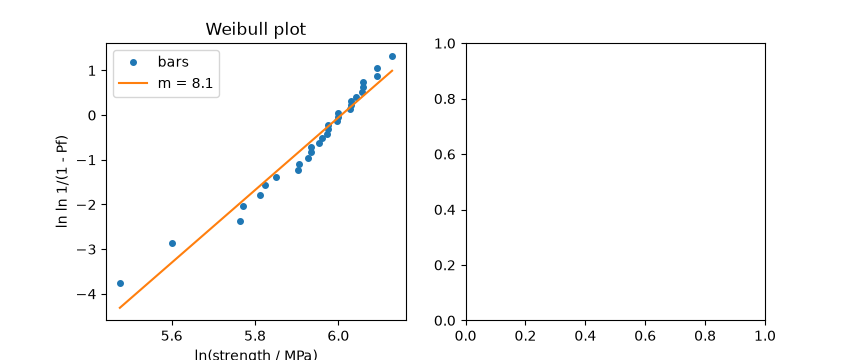
fitted m = 8.1, sigma_0 = 406 MPa, mean 383 MPa

<matplotlib.legend.Legend object at 0x7f9782c578c0>

Bigger parts are weaker

A component with 1000 times the stressed volume of a test bar has the same failure probability at a strength lower by \(1000^{1/m}\), a factor of 2 for \(m = 10\). Steels, with \(m\) above 30, hardly show the effect.

V_part = 1000 * V_test
part_strength = weibull_size_effect(sigma_0_fit, V_test, V_part, m_fit)
print(f"characteristic strength of the part: {part_strength / 1e6:.0f} MPa")
p_bar = weibull_failure_probability(250e6, sigma_0_fit, m_fit)
p_part = weibull_failure_probability(250e6, sigma_0_fit, m_fit, volume=V_part, reference_volume=V_test)
print(f"at 250 MPa: bar fails with probability {p_bar:.3f}, part with {p_part:.3f}")
assert np.isclose(weibull_failure_probability(part_strength, sigma_0_fit, m_fit, V_part, V_test), 1 - np.exp(-1))
assert p_part > p_bar

stress = np.linspace(50e6, 600e6, 200)
for V, label in ((V_test, "test bar"), (V_part, "part, 1000 V")):
    axs[1].plot(stress / 1e6, weibull_failure_probability(stress, sigma_0_fit, m_fit, V, V_test), label=label)
axs[1].set(xlabel="stress [MPa]", ylabel="failure probability", title="Size effect")
axs[1].legend()
fig.tight_layout()

plt.show()

characteristic strength of the part: 173 MPa
at 250 MPa: bar fails with probability 0.019, part with 1.000