Avrami’s transformation kinetics (1939)

Austenite turning to pearlite, cold-worked metal recrystallising and polymers crystallising all follow the same S-shaped curve. Melvin Avrami, then at Columbia, modelled nuclei that appear at random and grow until they run into each other: counting the “extended” volume they would fill if they could overlap, and removing the overlaps statistically, gives

\[y = 1 - e^{-kt^n}\]

(avrami_fraction()), with \(n\) between 1 and 4 set by how nucleation and growth proceed. Johnson and Mehl (1939) and Kolmogorov (1937) reached the same law. The example simulates nuclei on a grid, fits \(k\) and \(n\) (avrami_fit()), and uses the lever rule (lever_rule()) for the equilibrium amount of the new phase.

import matplotlib.pyplot as plt
import numpy as np

from engineeringkit.materials import avrami_fit, avrami_fraction, avrami_time, lever_rule

Random nuclei that impinge

In two dimensions, nuclei appear at a constant rate per unit area and grow as discs at constant speed. Those that land in already transformed material are Avrami’s “phantom” nuclei: they add nothing to the union of discs, which is why the extended-volume argument is exact. Avrami’s exponent is then \(n = 3\) (two for growth, one for nucleation).

rng = np.random.default_rng(1939)
size, rate, speed = 200, 2e-4, 1.0
yy, xx = np.mgrid[0:size, 0:size]
births = []
times = np.arange(1, 41)
fraction = []
transformed = np.zeros((size, size), bool)
for t in times:
    for _ in range(rng.poisson(rate * size * size)):
        births.append((rng.uniform(0, size), rng.uniform(0, size), t))
    transformed[:] = False
    for x0, y0, t0 in births:
        transformed |= (xx - x0) ** 2 + (yy - y0) ** 2 <= (speed * (t - t0)) ** 2
    fraction.append(transformed.mean())
fraction = np.array(fraction)

window = (fraction > 0.05) & (fraction < 0.95)
k, n = avrami_fit(times[window], fraction[window])
print(f"fitted k = {k:.2e} per step^n, n = {n:.2f}; half time {avrami_time(0.5, k, n):.1f} steps")
assert 2.7 < n < 3.3

fig, ax = plt.subplots(figsize=(6, 3.8))
ax.plot(times, fraction, "o", ms=4, label="simulated nuclei")
ax.plot(times, avrami_fraction(times, k, n), label=f"Avrami, n = {n:.2f}")
ax.set(xlabel="time [steps]", ylabel="fraction transformed", title="Nucleation and growth")
ax.legend()
fig.tight_layout()

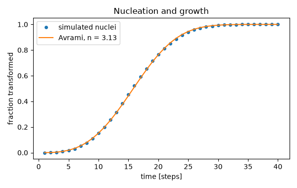
fitted k = 1.23e-04 per step^n, n = 3.13; half time 15.8 steps

How much forms: the lever rule

Kinetics says how fast; the phase diagram says how much. A 0.40 wt% C steel held just below the eutectoid line is ferrite (0.022 wt% C) and pearlite (0.76 wt% C); the tie line gives the pearlite fraction that the Avrami curve approaches.

W_ferrite, W_pearlite = lever_rule(0.40, 0.022, 0.76)
print(f"proeutectoid ferrite {W_ferrite:.2f}, pearlite {W_pearlite:.2f}")
assert np.isclose(W_ferrite * 0.022 + W_pearlite * 0.76, 0.40)

plt.show()

proeutectoid ferrite 0.49, pearlite 0.51