Huygens’s compound pendulum and the parallel-axis theorem (1673)

Christiaan Huygens (1673) asked how long a simple pendulum must be to swing in step with a rigid body pivoted at a point. His answer, the length \(L = I_O/(m d)\) to the centre of oscillation, needs the body’s moment of inertia about the pivot, which Jakob Steiner later wrote in general as \(I_O = I_G + m d^2\) (parallel_axis()). The example checks the theorem by summing \(r^2\,dm\) over a disk, recovers Huygens’s rule that pivot and centre of oscillation can be swapped without changing the period, and finds the correction he applied to a clock’s spherical bob.

import matplotlib.pyplot as plt
import numpy as np

from engineeringkit.integrators import integrate_ode
from engineeringkit.mechanical_engineering import angular_momentum, disk_inertia, parallel_axis, solid_sphere_inertia

g = 9.81

The parallel-axis theorem by direct summation

Cut a uniform disk into small squares and add up \(r^2\,dm\) about a pivot a distance \(d\) from the centre.

m, R = 2.0, 0.15
n = 1201
x, y = np.meshgrid(np.linspace(-R, R, n), np.linspace(-R, R, n))
inside = x**2 + y**2 <= R**2
dm = m / inside.sum()
for d in (0.0, 0.05, 0.10, 0.15):
    summed = np.sum(((x[inside] - d) ** 2 + y[inside] ** 2) * dm)
    steiner = parallel_axis(disk_inertia(m, R), m, d)
    print(f"d = {d:.2f} m: summed I = {summed:.6f}, I_G + m d^2 = {steiner:.6f} kg m^2")
    assert np.isclose(summed, steiner, rtol=2e-3)

d = 0.00 m: summed I = 0.022499, I_G + m d^2 = 0.022500 kg m^2
d = 0.05 m: summed I = 0.027499, I_G + m d^2 = 0.027500 kg m^2
d = 0.10 m: summed I = 0.042499, I_G + m d^2 = 0.042500 kg m^2
d = 0.15 m: summed I = 0.067499, I_G + m d^2 = 0.067500 kg m^2

Period of the disk pendulum and Huygens’s reciprocity

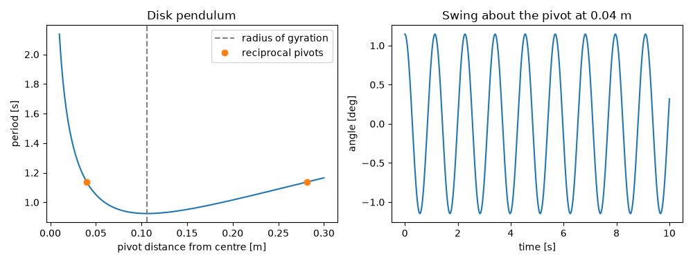
The period \(2\pi\sqrt{I_O/(m g d)}\) is smallest when the pivot sits at the radius of gyration \(k = R/\sqrt 2\). A pivot at the centre of oscillation, \(L - d\) on the other side of the centre, gives the same period: Kater’s reversible pendulum (1818) measured \(g\) this way.

d = np.linspace(0.01, 0.3, 300)
L = parallel_axis(disk_inertia(m, R), m, d) / (m * d)
period = 2 * np.pi * np.sqrt(L / g)
k = np.sqrt(disk_inertia(m, R) / m)
d1 = 0.04
L1 = parallel_axis(disk_inertia(m, R), m, d1) / (m * d1)
d2 = L1 - d1
L2 = parallel_axis(disk_inertia(m, R), m, d2) / (m * d2)
print(f"pivot {d1:.3f} m: L = {L1:.4f} m; pivot {d2:.4f} m: L = {L2:.4f} m")
assert np.isclose(L1, L2)
assert np.isclose(d[np.argmin(period)], k, atol=d[1] - d[0])

pivot 0.040 m: L = 0.3212 m; pivot 0.2812 m: L = 0.3212 m

Simulated swing

Integrate \(I_O\ddot\phi = -m g d \sin\phi\) at a small amplitude and time the zero crossings. The angular momentum \(I_O\dot\phi\) peaks as the disk passes the bottom.

I_O = parallel_axis(disk_inertia(m, R), m, d1)
t = np.linspace(0, 10, 20001)
swing = integrate_ode(lambda tt, s: [s[1], -m * g * d1 * np.sin(s[0]) / I_O], [0.02, 0.0], t)
phi = swing.history[:, 0]
crossings = t[1:][np.diff(np.sign(phi)) != 0]
measured = 2 * np.mean(np.diff(crossings))
print(f"simulated period {measured:.4f} s, Huygens 2 pi sqrt(L/g) = {2 * np.pi * np.sqrt(L1 / g):.4f} s")
print(f"peak angular momentum {np.max(angular_momentum(I_O, swing.history[:, 1])):.2e} kg m^2/s")
assert np.isclose(measured, 2 * np.pi * np.sqrt(L1 / g), rtol=1e-3)

simulated period 1.1371 s, Huygens 2 pi sqrt(L/g) = 1.1370 s
peak angular momentum 2.84e-03 kg m^2/s

The clock bob correction

A sphere of radius \(a\) on a light rod of length \(\ell\) beats as a simple pendulum of length \(\ell + \tfrac25 a^2/\ell\).

rod, a, bob = 0.994, 0.05, 1.0
L_bob = parallel_axis(solid_sphere_inertia(bob, a), bob, rod) / (bob * rod)
print(f"equivalent length {L_bob:.6f} m, correction {1e3 * (L_bob - rod):.3f} mm")
assert np.isclose(L_bob - rod, 0.4 * a**2 / rod)

fig, axes = plt.subplots(1, 2, figsize=(10, 3.8))
axes[0].plot(d, period)
axes[0].axvline(k, color="0.5", ls="--", label="radius of gyration")
axes[0].plot([d1, d2], [2 * np.pi * np.sqrt(L1 / g)] * 2, "o", label="reciprocal pivots")
axes[0].set(xlabel="pivot distance from centre [m]", ylabel="period [s]", title="Disk pendulum")
axes[0].legend()
axes[1].plot(t, np.degrees(phi))
axes[1].set(xlabel="time [s]", ylabel="angle [deg]", title=f"Swing about the pivot at {d1} m")
fig.tight_layout()

plt.show()

equivalent length 0.995006 m, correction 1.006 mm