Lagrange’s equations of motion (1788)

Joseph-Louis Lagrange’s Mécanique analytique (1788) contains no figures. It derives the motion of any system from two scalar functions, the kinetic energy \(T\) and the potential energy \(V\), written in whatever coordinates \(q\) fix its configuration. With \(L = T - V\),

\[\frac{d}{dt}\frac{\partial L}{\partial\dot q_i} - \frac{\partial L}{\partial q_i} = Q_i ,\]

and the constraint forces, such as the tension in a pendulum rod, never appear. lagrange_accelerations() evaluates these equations numerically from a Python function for \(L\), and simulate_lagrangian() integrates them. The example runs a double pendulum, checks it against the hand-derived equations and the conservation of energy, and linearises it to the small-oscillation eigenproblem Lagrange also set out.

import matplotlib.pyplot as plt
import numpy as np

from engineeringkit.mechanical_engineering import lagrange_accelerations, normal_modes, simulate_lagrangian

The double pendulum

Two point masses on rigid massless rods, angles \(\theta_1, \theta_2\) from the downward vertical.

m1, m2, l1, l2, g = 1.0, 1.0, 1.0, 1.0, 9.81


def lagrangian(q, v):
    T = 0.5 * (m1 + m2) * l1**2 * v[0] ** 2 + 0.5 * m2 * l2**2 * v[1] ** 2 + m2 * l1 * l2 * v[0] * v[1] * np.cos(q[0] - q[1])
    V = -(m1 + m2) * g * l1 * np.cos(q[0]) - m2 * g * l2 * np.cos(q[1])
    return T - V


q, v = np.array([2.0, 2.5]), np.array([0.0, 0.0])
d = q[0] - q[1]
H = np.array([[(m1 + m2) * l1**2, m2 * l1 * l2 * np.cos(d)], [m2 * l1 * l2 * np.cos(d), m2 * l2**2]])
rhs = [
    -m2 * l1 * l2 * v[1] ** 2 * np.sin(d) - (m1 + m2) * g * l1 * np.sin(q[0]),
    m2 * l1 * l2 * v[0] ** 2 * np.sin(d) - m2 * g * l2 * np.sin(q[1]),
]
by_hand = np.linalg.solve(H, rhs)
print("accelerations from L:", np.round(lagrange_accelerations(lagrangian, q, v), 6).tolist(), " by hand:", np.round(by_hand, 6).tolist())
assert np.allclose(lagrange_accelerations(lagrangian, q, v), by_hand, rtol=1e-6)

accelerations from L: [-10.316811, 3.182843]  by hand: [-10.316811, 3.182842]

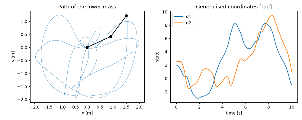
Chaotic motion that conserves energy

Released from high up, the motion is chaotic, but \(T + V\) stays constant; \(L(q, 0) = -V\).

t = np.linspace(0, 10, 2001)
run = simulate_lagrangian(lagrangian, q, v, t)
energy = np.array([lagrangian(a, b) - 2 * lagrangian(a, 0 * b) for a, b in zip(run.displacement, run.velocity)])
print(f"energy drift over 10 s: {np.ptp(energy) / abs(energy[0]):.1e} of the total")
assert np.ptp(energy) < 1e-5 * abs(energy[0])

energy drift over 10 s: 5.2e-07 of the total

Small oscillations

Near the hanging position \(T \approx \tfrac12\dot q^T M\dot q\) and \(V \approx \tfrac12 q^T K q\), so Lagrange’s equations become \(M\ddot q + Kq = 0\). Started in a normal mode, the pendulum returns to its start after one period.

M = np.array([[(m1 + m2) * l1**2, m2 * l1 * l2], [m2 * l1 * l2, m2 * l2**2]])
K = np.diag([(m1 + m2) * g * l1, m2 * g * l2])
modes = normal_modes(M, K)
print("small-oscillation periods [s]:", np.round(2 * np.pi / modes.frequencies, 4).tolist())
for shape, w in zip(modes.mode_shapes, modes.frequencies):
    small = simulate_lagrangian(lagrangian, 1e-3 * shape, [0.0, 0.0], np.linspace(0, 2 * np.pi / w, 101))
    assert np.allclose(small.displacement[-1], small.displacement[0], atol=1e-8)

x1, y1 = l1 * np.sin(run.displacement[:, 0]), -l1 * np.cos(run.displacement[:, 0])
x2, y2 = x1 + l2 * np.sin(run.displacement[:, 1]), y1 - l2 * np.cos(run.displacement[:, 1])
fig, (ax1, ax2) = plt.subplots(1, 2, figsize=(10, 4))
ax1.plot(x2, y2, lw=0.5)
ax1.plot([0, x1[0], x2[0]], [0, y1[0], y2[0]], "ko-")
ax1.set(aspect="equal", xlabel="x [m]", ylabel="y [m]", title="Path of the lower mass")
run.plot(ax=ax2)
ax2.set(title="Generalised coordinates [rad]")
fig.tight_layout()

plt.show()

small-oscillation periods [s]: [2.6211, 1.0857]