Rayleigh’s Theory of Sound: forced vibration and resonance (1877)

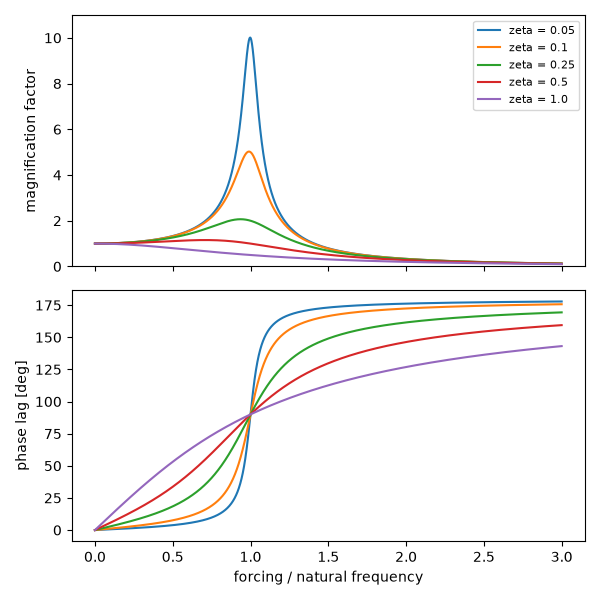
The third chapter of Rayleigh’s Theory of Sound drives the damped oscillator with a harmonic force, \(m\ddot x + c\dot x + kx = F_0\cos\omega t\). Once the free motion has died away the mass moves at the forcing frequency with amplitude \((F_0/k)\,M\), the static deflection times the magnification factor (magnification_factor()), and lags the force by a phase (phase_angle()) that passes through 90 degrees at \(\omega = \omega_n\) whatever the damping. Below resonance the spring carries the force, at resonance only damping limits the motion, and above it the mass’s inertia does. The example compares a simulated run-up of three forcing frequencies with the closed form.

import matplotlib.pyplot as plt
import numpy as np

from engineeringkit.mechanical_engineering import magnification_factor, phase_angle, simulate_sdof

Steady state of a simulated oscillator

After the transient decays, fit the amplitude and phase of the simulated displacement and compare them with \(M\) and \(\phi\).

m, k, c, F0 = 4.0, 1.6e4, 40.0, 100.0
wn, zeta = np.sqrt(k / m), c / (2 * np.sqrt(k * m))
t = np.linspace(0, 6, 60001)
tail = t > 4
for r in (0.5, 1.0, 2.0):
    w = r * wn
    x = simulate_sdof(m, c, k, t=t, force=lambda s, w=w: F0 * np.cos(w * s)).displacement
    basis = np.column_stack((np.cos(w * t[tail]), np.sin(w * t[tail])))
    a, b = np.linalg.lstsq(basis, x[tail], rcond=None)[0]
    amplitude, lag = np.hypot(a, b) / (F0 / k), np.arctan2(b, a)
    print(
        f"r = {r}: M = {amplitude:.4f} (closed form {magnification_factor(r, zeta):.4f}), "
        f"lag = {np.degrees(lag):.2f} deg (closed form {np.degrees(phase_angle(r, zeta)):.2f})"
    )
    assert np.isclose(amplitude, magnification_factor(r, zeta), rtol=1e-4)
    assert np.isclose(lag, phase_angle(r, zeta), atol=1e-4)

r = 0.5: M = 1.3260 (closed form 1.3260), lag = 6.02 deg (closed form 6.02)
r = 1.0: M = 6.3246 (closed form 6.3246), lag = 90.00 deg (closed form 90.00)
r = 2.0: M = 0.3315 (closed form 0.3315), lag = 173.98 deg (closed form 173.98)

Resonance curves

The peak, \(1/(2\zeta\sqrt{1 - \zeta^2})\), sits slightly below \(r = 1\); every phase curve crosses 90 degrees at \(r = 1\).

r = np.linspace(0, 3, 3001)
fig, (ax1, ax2) = plt.subplots(2, 1, sharex=True, figsize=(6, 6))
for z in (0.05, 0.1, 0.25, 0.5, 1.0):
    ax1.plot(r, magnification_factor(r, z), label=f"zeta = {z}")
    ax2.plot(r, np.degrees(phase_angle(r, z)))
    if z < 1 / np.sqrt(2):
        assert np.isclose(magnification_factor(r, z).max(), 1 / (2 * z * np.sqrt(1 - z * z)), rtol=1e-3)
    assert np.isclose(phase_angle(1.0, z), np.pi / 2)
ax1.set(ylabel="magnification factor", ylim=(0, 11))
ax1.legend(fontsize=8)
ax2.set(xlabel="forcing / natural frequency", ylabel="phase lag [deg]")
fig.tight_layout()

plt.show()