Dunkerley’s whirling shafts and Rayleigh’s bound (1894)

Stanley Dunkerley measured the whirling speeds of shafts carrying pulleys at Owens College, Manchester, and found an empirical rule: the inverse squares of the critical speeds of each pulley alone, and of the bare shaft, add up to the inverse square of the critical speed of the whole, \(1/\omega^2 \approx \sum_i 1/\omega_i^2\) (dunkerley_frequency()). The sum is the trace of the flexibility-mass matrix, the sum of the inverse squares of every natural frequency, so it always underestimates the fundamental. Rayleigh’s quotient with the static deflection as the trial shape (rayleigh_frequency()) always overestimates it. The example brackets the first critical speed of a simply supported shaft with three disks.

import matplotlib.pyplot as plt
import numpy as np

from engineeringkit.mechanical_engineering import dunkerley_frequency, normal_modes, rayleigh_frequency

Influence coefficients of a simply supported shaft

The deflection at \(x\) due to a unit load at \(a\) on a span \(L\) is \(b x (L^2 - b^2 - x^2)/(6EIL)\) for \(x \le a\), \(b = L - a\). The shaft itself is taken as massless, so Dunkerley’s bare-shaft term is zero.

E, d, L = 207e9, 0.05, 1.2
I = np.pi * d**4 / 64
stations = np.array([0.3, 0.6, 0.9])
masses = np.array([20.0, 35.0, 15.0])


def influence(x, a):
    if x > a:
        x, a = L - x, L - a
    b = L - a
    return b * x * (L**2 - b**2 - x**2) / (6 * E * I * L)


A = np.array([[influence(x, a) for a in stations] for x in stations])
assert np.allclose(A, A.T)  # Maxwell's reciprocal theorem

Bounds and the exact value

M, K = np.diag(masses), np.linalg.inv(A)
exact = normal_modes(M, K).frequencies[0]
static = A @ (masses * 9.81)
upper = rayleigh_frequency(M, K, static)
lower = dunkerley_frequency(masses, A)
alone = 1 / np.sqrt(masses * np.diag(A))
rpm = 60 / (2 * np.pi)
print(f"each disk alone [rpm]: {np.round(alone * rpm).tolist()}")
print(f"Dunkerley {lower * rpm:.0f} rpm <= exact {exact * rpm:.0f} rpm <= Rayleigh {upper * rpm:.0f} rpm")
assert lower < exact < upper
assert np.isclose(1 / lower**2, np.sum(1 / alone**2))
assert upper / exact - 1 < 1e-3 and 1 - lower / exact < 0.05

each disk alone [rpm]: [3781.0, 2144.0, 4366.0]
Dunkerley 1715 rpm <= exact 1761 rpm <= Rayleigh 1761 rpm

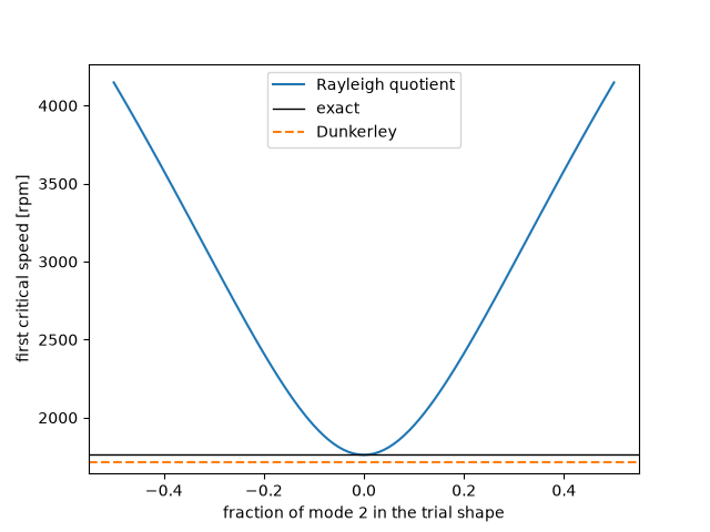
Rayleigh’s quotient is stationary at the mode

Mixing a fraction \(\varepsilon\) of the second mass-normalised mode into the first gives exactly \(\omega^2 = (\omega_1^2 + \varepsilon^2\omega_2^2)/(1 + \varepsilon^2)\): a 10% error in the shape costs only about 1% of \(\omega_2^2 - \omega_1^2\).

phi, w = normal_modes(M, K).mode_shapes, normal_modes(M, K).frequencies
eps = np.linspace(-0.5, 0.5, 101)
estimate = np.array([rayleigh_frequency(M, K, phi[0] + e * phi[1]) for e in eps])
assert np.all(estimate >= exact * (1 - 1e-12))
assert np.allclose(estimate**2, (w[0] ** 2 + eps**2 * w[1] ** 2) / (1 + eps**2))

fig, ax = plt.subplots()
ax.plot(eps, estimate * 60 / (2 * np.pi), label="Rayleigh quotient")
ax.axhline(exact * 60 / (2 * np.pi), color="k", lw=1, label="exact")
ax.axhline(lower * 60 / (2 * np.pi), color="C1", ls="--", label="Dunkerley")
ax.set(xlabel="fraction of mode 2 in the trial shape", ylabel="first critical speed [rpm]")
ax.legend()

plt.show()